Soft Actor Critic (Visualized) : From Scratch in Torch for Inverted Pendulum

Introduction

In this post, I will implement the Soft Actor Critic (SAC) algorithm from scratch in PyTorch. I will use the OpenAI Gym environment for the Inverted Pendulum task.
The goal of this post is to provide a Torch code follow along for the original paper by Haarnoja et al. (2018) [1]. Many implementations of Soft Actor Critic exist, in this code we implement the one outlines in the paper.
You can follow along by starting from main_sac.py at the following link:
https://github.com/FranciscoRMendes/soft-actor-critic

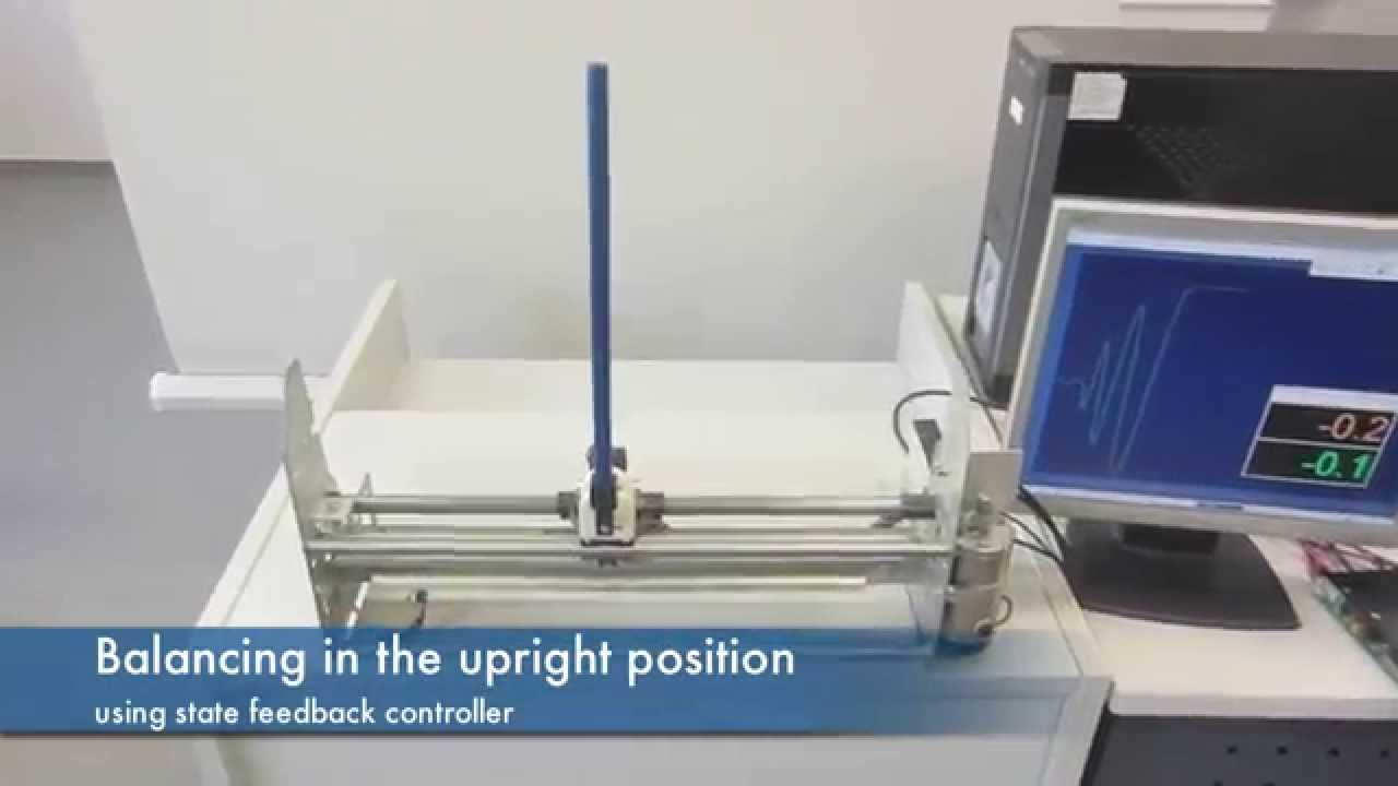
Inverted Pendulum v0 Environment Set Up

Environment Set Up

Link to the environment here : https://github.com/bulletphysics/bullet3/blob/master/examples/pybullet/gym/pybullet_envs/gym_pendulum_envs.py

Example Data

The data from playing the game looks something like this, with each instant of game play denoted by a row. Note this data is sampled from many different games, so it is not ordered as if coming from one game.
The dashes in the column name denote the next state, for example, Position’ is the position at the next time step.

Position	Velocity	Cos Pole Angle	Sine Pole Angle	Pole Angle	Time Step	Force L/R	Position’	Velocity’	Cos Pole Angle’	Sine Pole Angle’	Pole Angle’	Done
0.0002	0.0085	0.9974	-0.0722	-0.0647	1	0.0137	0.0004	0.0133	0.9973	-0.0738	-0.0985	FALSE
0.0174	0.0954	0.9964	-0.0842	-0.4624	1	0.0389	0.0191	0.1039	0.9957	-0.0926	-0.5079	FALSE
0.0031	0.0427	0.9969	-0.0785	-0.2768	1	0.0290	0.0040	0.0497	0.9965	-0.0837	-0.3173	FALSE
0.0046	0.0540	0.9965	-0.0840	-0.3380	1	0.0327	0.0056	0.0617	0.9959	-0.0902	-0.3818	FALSE
0.0008	0.0195	0.9967	-0.0813	-0.1428	1	0.0203	0.0012	0.0255	0.9964	-0.0843	-0.1822	FALSE
0.0071	0.0438	0.9994	-0.0359	-0.1959	1	0.0196	0.0079	0.0478	0.9992	-0.0395	-0.2158	FALSE
0.0133	0.1056	0.9928	-0.1194	-0.6067	1	0.0512	0.0153	0.1171	0.9915	-0.1304	-0.6702	FALSE

State Description in InvertedPendulumBulletEnv-v0

1. Cart Position – The horizontal position of the cart.
2. Cart Velocity – The speed of the cart.
3. Cosine of Pendulum Angle – , where is the angle relative to the vertical. It equals 1 when upright and decreases as it tilts.
4. Sine of Pendulum Angle – complements , providing a full representation of the angle.
5. Pendulum Angular Velocity – The rate of change of .

Action

The action space is continuous and consists of a single action that can be applied to the cart. The action is a force that can be applied to the cart in the left or right direction. The force can be any value between and .

Reward & Termination

The reward is for every time step the pole is upright. The episode ends (Done is TRUE) when the pole is more than degrees from the vertical axis or the cart moves more than units from the center.

Game play GIF

An example of game play would look like this, not the most exciting thing in the world, I know.

The Neural Networks in Soft Actor Critic Network

The Lucid chart below encapsulates the major neural networks in the code and their relationships. Forward relationships (i.e. forward pass) are given by solid arrows. While backward relationships (i.e. backpropagation) are given by dashed arrows.
I recommend using this chart to keep a track of which outputs train which networks. Note however, that these backward arrows describe merely that some relationship exists. There are differences in the backpropagation used to train the policy network itself (uses the reparameterization trick) and the Value networks (does not).

The main object in the code is the object called SoftActorCritic.py. It consists of the neural networks and all the hyperparameters that potentially need tuning. As per the paper the most important one is reward scale. This is a hyperparameter that balances the explore-exploit tradeoff. Higher values of the reward will make the agent exploit more.

This class contains the following Neural Networks, their relationships are illustrated in the Lucid Chart above:

1. self.pi_phi: The actor network, which outputs the action given the state. In the paper this is denoted by the function , where is the policy, are the parameters of the policy, is the action at time , and is the state at time . This neural network will take in the state vector in this case the dimensional state vector, it can output two things
   • action : a continuous vector of size to take in the environment (no re-parameterization trick)
   • The mean and variance of the action to take in the environment, and respectively (re-parameterization trick)
2. self.Q_theta_1 : The first Q-network, this is also known as the critic network. It takes in the state and action as input and outputs the Q-value. In the paper this is denoted by the function , where is the Q-function, are the parameters of the first Q-network, is the state at time , and is the action at time .
3. self.Q_theta_2 : The second Q-network, this is also known as the critic network. It takes in the state and action as input and outputs the Q-value. In the paper this is denoted by the function , where is the Q-function, are the parameters of the second Q-network, is the state at time , and is the action at time .
4. self.V_psi : The Value network parameterized by in the paper. It takes in the state as input and outputs the value of the state. In the paper this is denoted by the function , where is the value function, are the parameters of the value network, and is the state at time .
5. self.V_psi_bar : The target value parameterized by in the paper. It takes in the state as input and outputs the value of the state. In the paper this is denoted by the function , where is the value function, are the parameters of the target value network, and is the state at time .

Couple of things to watch out for in these neural networks that can be quite different from the usual classification use,

1. Forward pass and inference (i.e. using the SoftActorCritic Network) are different, in the forward pass you are still using outputs to improve the policy network so that it plays better. However, to play the game you only ever need the policy network. In the classification case, the forward pass and inference are the same and hence used interchangeably.
2. The backward dashed arrows for backpropagation are important because it is not always clear what the “target” to train one of these neural networks is. The “target” is often from a combination of outputs from different networks and the rewards.
3. The top row of nodes, States, Actions, Rewards and Next States are the “data” on which the neural networks are to be trained.

   class SoftActorCritic:
       def __init__(self, alpha=0.0003, beta=0.0003, input_dims=[8],
                    env=None, gamma=0.99, n_actions=2, max_size=1000000, tau=0.005, batch_size=256, reward_scale=2):
           self.gamma = gamma
           self.tau = tau
           self.memory = ReplayBuffer(max_size, input_dims, n_actions)
           self.batch_size = batch_size
           self.n_actions = n_actions
           self.pi_phi = ActorNetwork(alpha, input_dims, n_actions=n_actions, name='actor', max_action=env.action_space.high) # 1
           self.Q_theta_1 = CriticNetwork(beta, input_dims, n_actions=n_actions, name='critic_1')
           self.Q_theta_2 = CriticNetwork(beta, input_dims, n_actions=n_actions, name='critic_2')
           self.V_psi = ValueNetwork(beta, input_dims, name='value')
           self.V_psi_bar = ValueNetwork(beta, input_dims, name='target_value')
           self.scale = reward_scale # You will find this in the ablation study section of the paper this balances the explore/exploit tradeoff
           self.update_psi_bar_using_psi(tau=1)

Learning in SAC

The learning in the model is handled by the learn function. This function takes in the batch of data from the replay buffer and updates the parameters of the networks. The learning is done in the following steps:

1. Sample a batch of data from the replay buffer. If the data is not enough i.e. smaller than batch size, return.
2. Optimize the Value Network using the soft Bellman equation (equation )
3. Optimize the Policy Network using the policy gradient (equation )
4. Optimize the Q Network using the Bellman equation (equation )

Couple of asides here,

1. The words network and function can be used interchangeably. The neural network serves as a function approximator for the functions we are trying to learn (Value, Q, Policy).
2. The Value Networks and Policy Networks are dependent on the current state of the Q network. Only after these are updated can we update the Q network.
3. All loss functions are denoted by in the paper. The subscript denotes the network that is being optimized. For example, is the loss function for the Value Network, is the loss function for the Policy Network, and is the loss function for the Q Network.
4. The Target Network is simply a lagged duplicate of the current Value Network. Thus, it does not actually ever “learn” but simply updates it weights through a weighted average between the latest weights from the value network and its own weights, this is given by the parameter in the code. This is done to stabilize the learning process.
5. Variable names can be read as one would read the variable from the paper for instance is given by V_psi_bar_s_t_plus_1. It is unfortunate that python does not allow for more scientific notation, but this is the best I could do.

Re-parameterization Trick

One of the most confusing things to implement in python. You can skip this section if you are just starting out but its use will become clear later. Adding the details here for completeness.

The main problem we are trying to solve here is that Torch requires a computational graph to perform backpropagation of the gradients. rsample() preserves the graph information whereas sample() does not. This is because rsample() uses the reparameterization trick to sample from the distribution. The reparameterization trick is a way to sample from a distribution while preserving the gradient information. It is done by expressing the random variable as a deterministic function of a parameter and a noise variable. In this case, we are using the reparameterization trick to sample from the normal distribution. The normal distribution is parameterized by its mean and standard deviation. We can express the random variable as a deterministic function of the mean, standard deviation, and a noise variable. This allows us to sample from the distribution while preserving the gradient information.

1. sample(): Performs random sampling, cutting off the computation graph (i.e., no backpropagation). Uses torch.normal within torch.no_grad(), ensuring the result is detached.
2. rsample(): Enables backpropagation using the reparameterization trick, separating randomness into an independent variable (eps). The computation graph remains intact as the transformation (loc + eps * scale) is differentiable.

Key Idea: eps is sampled once and remains fixed, while loc and scale change during optimization, allowing gradients to flow. Used in algorithms like SAC (Soft Actor-Critic) for reinforcement learning.
If you want to sample both the values and plot their distributions they will be identical (or as identical as two samples sampled from the same distribution can be).

A good explanation can be found here : https://stackoverflow.com/questions/60533150/what-is-the-difference-between-sample-and-rsample

def sample_normal(self, state, reparameterize=True):
    mu, sigma = self.forward(state)
    probabilities = Normal(mu, sigma)

    if reparameterize:
        actions = probabilities.rsample()
    else:
        actions = probabilities.sample()

    action = T.tanh(actions)*T.tensor(self.max_action).to(self.device)
    log_probs = probabilities.log_prob(actions)
    log_probs -= T.log(1-action.pow(2)+self.reparam_noise)
    log_probs = log_probs.sum(1, keepdim=True)

    return action, log_probs

Learning the Value Function

With all the caveats and fine print out of the way we can begin the learn function.
Here we take a sample of data from the replay buffer. Now recall, that we need to take a random sample and not just the values because the data is not i.i.d. and we need to break the correlation between the data points.

sample = self.memory.sample_buffer(self.batch_size)
s_t, a_t_rb, r_t, s_t_plus_1, done = self.process_sample(sample, self.pi_phi.device)

Let us first state the loss function of the value function. This is equation 5 of the Haarnoja et al. (2018) paper.

Comments,

1. is the output of the value function, which would just be a forward pass through the value neural network denoted by self.V_psi(s_t) in the code.
2. is the output of the target value function, which would just be a forward pass through the target value neural network for the next state denoted by self.V_psi_bar(s_t_plus_1) in the code.
3. We also need the output of the Q function, which would just be a forward pass through the Q neural network denoted by self.Q_theta_1.forward(s_t, a_t) in the code. But since we have two Q networks, we need to take the minimum of the two. This is done to reduce the overestimation bias in the Q function.

V_psi_s_t = self.V_psi(s_t).view(-1)

V_psi_bar_s_t_plus_1 = self.V_psi_bar(s_t_plus_1).view(-1)

V_psi_bar_s_t_plus_1[done] = 0.0

a_t_D, log_pi_t_D = self.pi_phi.sample_normal(s_t, reparameterize=False) # here we are not using the reparameterization trick because we are not backpropagating through the policy network

log_pi_t_D = log_pi_t_D.view(-1)

# Find the value of the Q function for the current state and action, since we have two networks we take the minimum of the two
Q_theta_1_s_t_a_t_D = self.Q_theta_1.forward(s_t, a_t_D)
Q_theta_2_s_t_a_t_D = self.Q_theta_2.forward(s_t, a_t_D)
Q_theta_min_s_t_a_t_D = T.min(Q_theta_1_s_t_a_t_D, Q_theta_2_s_t_a_t_D)
# This is the Q value to be used in equation 5
Q_theta_min_s_t_a_t_D = Q_theta_min_s_t_a_t_D.view(-1)

self.V_psi.optimizer.zero_grad()
# This is exactly equation 5
J_V_psi = 0.5 * F.mse_loss(V_psi_s_t, Q_theta_min_s_t_a_t_D - log_pi_t_D)
J_V_psi.backward(retain_graph=True) # again, we don't need to backpropagate through the policy network
self.V_psi.optimizer.step() # Update the value network

Learning the Policy Function

The policy function is learned using the policy gradient. This is equation 12 of the Haarnoja et al. (2018) paper.

The expectation means that we can use the mean of the observed values to approximate the expectation.
For performing the optimization on the policy network we need to do two things to get a prediction,

1. Perform a forward pass through the network to get and .
2. Sample an action from the policy network using the reparameterization trick. This ensures that the computational graph is preserved and we can backpropagate through the policy network. This was not true in the previous case.
   Here it may seems like the values for and are the same as the ones we used for the value function. This is not the case, we need to sample a new action from the policy network and use that to compute the Q value and log probability. This is because we are trying to learn the policy function, which is a stochastic process. We need to sample a new action from the policy network and use that to compute the Q value and log probability. This is done using the reparameterization trick.

# a_t_D refers to actions drawn from a sample of the actor network and not the true actions taken from the replay buffer
a_t_D, log_pi_t_D = self.pi_phi.sample_normal(s_t, reparameterize=True) # here we are using the reparameterization trick because we are backpropagating through the policy network
log_pi_t_D = log_pi_t_D.view(-1)
Q_theta_1_s_t_a_t_D = self.Q_theta_1.forward(s_t, a_t_D)
Q_theta_2_s_t_a_t_D = self.Q_theta_2.forward(s_t, a_t_D)
Q_theta_min_s_t_a_t_D = T.min(Q_theta_1_s_t_a_t_D, Q_theta_2_s_t_a_t_D)
Q_theta_min_s_t_a_t_D = Q_theta_min_s_t_a_t_D.view(-1)

# This is equation 12 in the paper
# note that this is identical to the original loss function given by equation 10
# after doing the re-parameterization trick
J_pi_phi = T.mean(log_pi_t_D - Q_theta_min_s_t_a_t_D)
self.pi_phi.optimizer.zero_grad()
J_pi_phi.backward(retain_graph=True)
self.pi_phi.optimizer.step()

Learning the Q-Network

In this section we will optimize the critic network. This would correspond to equation 7 in the paper.

Noting that,

This is somewhat different from equation 7 in the paper,

1. First, does not depend on in this case. This is because we are using the Inverted Pendulum environment, which gives a constant reward for each step.
2. Second, we drop the expectation over because we are using a single sample from the replay buffer for each (technically you should take the mean over multiple but this is a good enough approximation).
3. We use the actual actions taken from the replay buffer to compute the Q value. This is because we are trying to learn the Q function, which is a deterministic process. We need to use the actual actions taken from the replay buffer to compute the Q value. This is given by a_t_rb in the code.
4. We have two Q networks so we need to apply this individually to both networks.

# In this section we will optimize the two critic networks
# We will use the bellman equation to calculate the target Q value
self.Q_theta_1.optimizer.zero_grad()
self.Q_theta_2.optimizer.zero_grad()
# Equation 8 in the paper, in the paper the reward also depends on a_t
# but in this case we get a constant reward for each step, so we can just use r_t
# consequently, Q_hat_s_t AND NOT Q_hat_s_t_a_t
Q_hat_s_t = self.scale*r_t + self.gamma*V_psi_bar_s_t_plus_1
Q_theta_1_s_t_rb_at = self.Q_theta_1.forward(s_t, a_t_rb).view(-1) # this is the only place where actions from the replay buffer are used
Q_theta_2_s_t_rb_at = self.Q_theta_2.forward(s_t, a_t_rb).view(-1)
# this is equation 7 in the paper, one for each Q network
J_Q_theta_1_loss = 0.5 * F.mse_loss(Q_theta_1_s_t_rb_at, Q_hat_s_t)
J_Q_theta_2_loss = 0.5 * F.mse_loss(Q_theta_2_s_t_rb_at, Q_hat_s_t)
J_Q_theta_12 = J_Q_theta_1_loss + J_Q_theta_2_loss
J_Q_theta_12.backward()
self.Q_theta_1.optimizer.step()
self.Q_theta_2.optimizer.step()

Learning the target value network

The final piece of this puzzle is learning of the target value network. Now, there is no actual “learning” taking place in this network.
This network is simply a weighted lagged duplicate of the current value network. Thus, it does not actually ever “learn” but simply updates it weights through a weighted average between the latest weights from the value network and its own weights, this is given by the parameter in the code. This is done to stabilize the learning process.
This takes place in the line self.update_psi_bar_using_psi(tau=None) of the learn function.
The parameter tau is used to weight the copying, with tau = 1 being a complete copy and tau = 0 being no copy. Obviously for the learning to take place tau>0 but usually a vale of is used.
This function corresponds to the last line in the algorithm,

def update_psi_bar_using_psi(self, tau=None):
    # This function corresponds to the update step inside algorithm 1
    # this is the last line in the algorithm
    # psi_bar = tau* psi + (1-tau)*psi_bar
    if tau is None:
        tau = self.tau

    psi_bar = self.V_psi_bar.named_parameters()
    psi = self.V_psi.named_parameters()

    target_value_state_dict = dict(psi_bar)
    value_state_dict = dict(psi)

    for name in value_state_dict:
        value_state_dict[name] = tau*value_state_dict[name].clone() + (1-tau)*target_value_state_dict[name].clone()

    self.V_psi_bar.load_state_dict(value_state_dict)

Conclusion

This post has been a detailed walk through of the Soft Actor Critic algorithm using inverted pendulum as an example. Other implementations of this algorithm exist. The best one I have found is Phil Tabor’s implementation.
However, there was not a very good connection between the code and the paper. This post was an attempt to bridge that gap by using notation that exactly matches the paper, while keeping the overall structure simple to understand.
In my next post, I will implement the Soft Actor Critic Algorithm on the Lunar Lander game, this will hopefully make for a more interesting visualization of how the algorithm learns better.

References

1. Haarnoja, T., Zhou, A., Abbeel, P., & Levine, S. (2018). Soft Actor-Critic: Off-Policy Maximum Entropy Deep Reinforcement Learning with a Stochastic Actor. arXiv preprint arXiv:1801.01290.
2. https://github.com/philtabor/Youtube-Code-Repository/tree/master/ReinforcementLearning/PolicyGradient/SAC
3. Phil’s Youtube video https://www.youtube.com/watch?v=ioidsRlf79o
4. Oliver Sigaud’s video https://www.youtube.com/watch?v=_nFXOZpo50U (check out his channel and research for more)
5. https://youtube.com/playlist?list=PLYpLNGpDoiMSMrvgVhgNRwOHTVYbX2lOa&si=unvWxJsJm_w4OcD-
6. https://www.youtube.com/watch?v=kJ9CL7asR94&list=LL&index=22&t=41s (accent might be unclear, but trust me one of the best videos)