From Bits to Clocks: A Visual Intuition for the Quantum Fourier Transform
Introduction
Sometimes it does seem like my blog is just increasingly complex applications of the Fourier Transform. In the previous post we applied the Fourier Transform to graphs, drawing connections between frequency (which is the usual Fourier transform) and properties of the graph. There is yet another interesting, if abstract, application of the Fourier transform that is used in Quantum computers. Somewhat surprisingly, it is called the “Quantum Fourier Transform”. More specifically, we will study how the Fourier Transform appears as a unitary linear operator acting on quantum states.
At the end of the day this is all just linear algebra, requiring no knowledge of actual quantum physics. Because the Quantum Fourier Transform can be somewhat mathematically abstract and also because the Fourier Transform is so easily visualized as a decomposition into various sines and cosines, I thought of coming up with a similar visualization for the Quantum Fourier Transform case (spoiler: it involves clocks).
Motivation
\section{Motivation}
Before discussing in detail what the QFT is mathematically, it is useful to recap what the Fourier transform is in general. The Fourier transform is a way of transforming information from one domain to another domain. Why? Because certain operations become simpler in the transformed domain. For example, in classical signal processing, convolution of a signal (the mathematical definition of filtering) in the time domain corresponds to simple multiplication in the frequency domain.
In the graph setting, we saw that potentially complex behaviors in the edge-node representation of the graph were far more mathematically tractable when looking at the “frequency” equivalent of the graph. Eigenvectors of the graph Laplacian isolate modes of variation: low-frequency components capture global structure, while high-frequency components capture local fluctuations.
Similarly, for the Quantum Fourier Transform, we move from a bit representation of a number to a cyclical or phase representation. In the computational basis, information is stored as binary digits, essentially a sequence of ON/OFF switches taking values in
In this form, the data is linear and rigid. Any underlying periodic structure is hidden inside the positional encoding. Phases, however, live on the circle and are inherently cyclical. If we want to detect periodicity or modular structure, it is more natural to encode information as rotations rather than switches.
The QFT therefore plays the same conceptual role as the classical Fourier transform: it changes coordinates to a representation in which the problem’s hidden structure becomes easier to manipulate.
I might do a post later on why this is true on so many different problems. But it is not true for some problems such as when you need convolution to learn a local filter.
Useful Intuition
One of the reasons the Fourier transform in its simplest form is so
interesting is that it is so visual. Consider below the Fourier
transform on a simple 1-D wave (pulled from the internet) and a Fourier
Transform (from yours truly).


In this blog post I will try to provide a nice visual explanation for
the QFT. Essentially we want to draw a connection between the binary
representation of a number and the cyclical nature of the QFT.
Fortunately, there is a nice visual representation for a binary
representation of a number on a computer, called a qubit. This
representation of a number is called a qubit.
A Useful Visualization