Bayesian A/B Testing Is Not Immune to Peeking: Insights from the AV Marketplace
- Bayesian Statistics : A/B Testing, Thompson sampling of multi-armed bandits, Recommendation Engines and more from Big Consulting
- The Management Consulting Playbook for AB Testing (with an emphasis on Recommender Systems)
- No, You Cannot RCT Your Way to Policy
- Bayesian A/B Testing Is Not Immune to Peeking: Insights from the AV Marketplace
The Setup
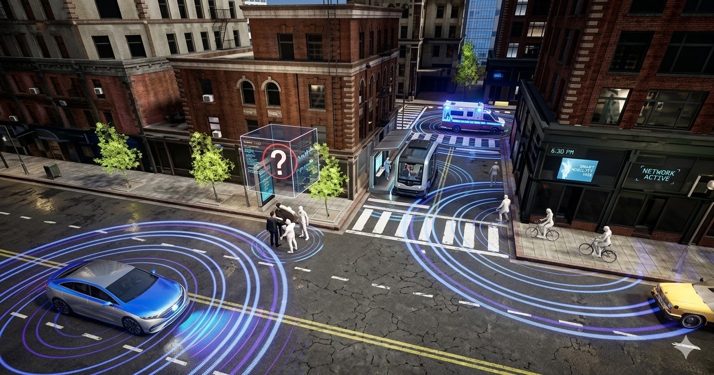
Imagine you are running an experiment to test the efficacy of a rewards program built to incentivize the use of autonomous vehicles in a ride-share marketplace. AVs cost more to operate than driver cars, so the business case depends heavily on whether riders can be nudged toward them at sufficient volume. The rewards program is the nudge — discounts, points, whatever it takes — and you need to know if it works.
The catch is that the rewards program itself costs money for every day it runs. Every subsidised ride is a line item. So there is real pressure to end the experiment as early as possible. Enter some Bayesian fanatic who proposes the solution: run a Bayesian experiment instead of a frequentist one. The argument is that Bayesian methods allow you to check results continuously and stop the moment you have sufficient evidence, which would dispense entirely with the need for a fixed sample size, the indignity of waiting, and crucially the problem of peeking.
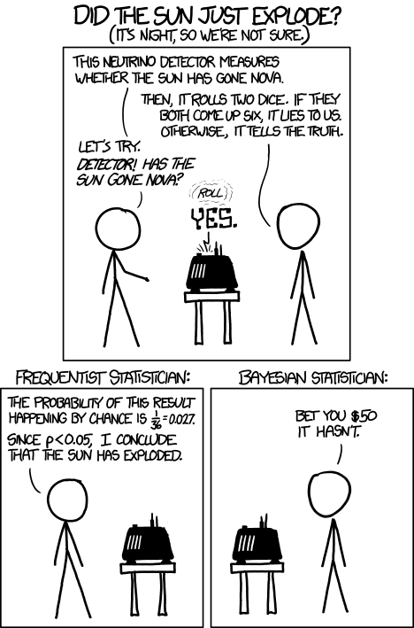
The Bayesian in this comic is right about priors. The Bayesian in our meeting was right about priors too. Neither of them was right about the experiment being cheap.
My disagreement was vigorous enough that simply asserting it felt insufficient, and so I brought the math, which has the considerable advantage of being harder to dismiss than mere opinion.
Frequentist Sample Size
To set the baseline, here is the standard frequentist formulation. We are testing whether the rewards program (arm B) increases AV ride take-rate relative to no rewards (arm A), where $\theta$ is the probability a rider chooses an AV:
$$ H_0: \theta_A = \theta_B, \quad H_1: \theta_B > \theta_A $$With Type I error $\alpha$ and power $1-\beta$, the required sample size per arm is:
$$ n_\text{freq} = \frac{\left( z_{1-\alpha/2} + z_{1-\beta} \right)^2 \left[ \theta_A (1-\theta_A) + \theta_B (1-\theta_B) \right]}{(\theta_B - \theta_A)^2} $$where $z_q$ denotes the $q$-th quantile of the standard normal distribution. The numerator grows with the variance of each arm; the denominator shrinks with the effect size squared. If the rewards program moves the AV take-rate only slightly, you need a very large experiment. This was, in fact, the source of the cost anxiety — the expected lift was small, which meant the required sample size was large, which meant the rewards program would run for a long time at a loss.
This is the formula the Bayesian fanatic wanted to escape. On to the proposed alternative.
Bayesian Sample Size
The Bayesian formulation replaces the frequentist error guarantees with a posterior expected loss criterion. We approximate the posterior on each arm’s conversion rate as Gaussian — reasonable for proportions with sufficient data:
$$ \theta_A \mid D_A \sim \mathcal{N}(\hat{\theta}_A, \sigma_A^2), \quad \theta_B \mid D_B \sim \mathcal{N}(\hat{\theta}_B, \sigma_B^2) $$with posterior variances:
$$ \sigma_A^2 \approx \frac{\hat{\theta}_A (1-\hat{\theta}_A)}{n}, \quad \sigma_B^2 \approx \frac{\hat{\theta}_B (1-\hat{\theta}_B)}{n} $$Instead of controlling Type I error, we set a threshold $\epsilon$ on the probability of selecting the wrong arm:
$$ p_\text{wrong} = \mathbb{P}(\text{choose wrong arm}) < \epsilon $$Solving for $n$, the required sample size per arm is:
$$ n_\text{bayes} = \frac{\hat{\theta}_A (1-\hat{\theta}_A) + \hat{\theta}_B (1-\hat{\theta}_B)}{(\hat{\theta}_B - \hat{\theta}_A)^2} \cdot \left[ \Phi^{-1}(1-\epsilon) \right]^2 $$where $\Phi^{-1}$ is the inverse standard normal CDF. Look at the structure. It is identical to the frequentist formula. The variance terms are the same. The effect size in the denominator is the same. The only difference is the squared prefactor: $\left[\Phi^{-1}(1-\epsilon)\right]^2$ instead of $\left(z_{1-\alpha/2} + z_{1-\beta}\right)^2$.
Example
Put some numbers on it. Suppose the baseline AV take-rate is 50% and the rewards program is expected to lift it by 2 percentage points:
- $\theta_A = 0.50$, $\theta_B = 0.52$
- Frequentist: $\alpha = 0.05$, power $= 0.8$ $\implies z_{1-0.025} + z_{0.8} \approx 1.96 + 0.84 = 2.8$
- Bayesian: $\epsilon = 0.05 \implies \Phi^{-1}(0.95) \approx 1.645$
Setting aside the variance terms, which are identical for both, the sample sizes scale as:
$$ n_\text{freq} \propto (2.8)^2 = 7.84, \quad n_\text{bayes} \propto (1.645)^2 = 2.71 $$On paper, the Bayesian approach needs roughly a third of the frequentist sample. If you are the person trying to minimise the cost of subsidising AV rides, this looks like exactly what you wanted, and it is the kind of result that tends to end conversations in rooms where people are more motivated by the cost of the experiment than the integrity of it. It is also, as it turns out, not quite right.
Bayesian Is Not Immune to Peeking
The critical assumption buried in the Bayesian sample size formula is that you collect $n_\text{bayes}$ samples and then evaluate the stopping criterion. You do not evaluate it after every ride. You do not check it at the end of each day because finance is asking. You do not peek.
Peeking is the practice of inspecting results before the planned sample size is reached and stopping early if the numbers look good. It is what invalidates frequentist tests when p-values are checked repeatedly mid-experiment — the false positive rate inflates because you are effectively running multiple tests and keeping the best result. The same logic applies to the Bayesian posterior.
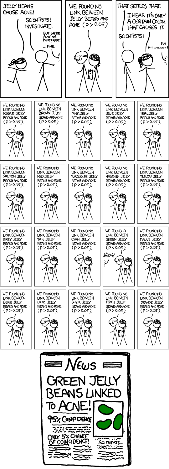
Run enough tests, check often enough, and green jelly beans will cause acne. The Bayesian equivalent: check the posterior enough times and your rewards program will appear to work. The AV subsidy line item does not care which framework licensed your false positive.
If you evaluate $p_\text{wrong} < \epsilon$ continuously and stop the moment it dips below threshold, you have not run the experiment described by the formula above. You have run something different, with different — and worse — statistical properties. The Bayesian framing does not make this problem disappear. It reframes it. The stopping rule is still a rule, and it must be respected as such.
The Deeper Point
Now consider what happens when you align the frequentist and Bayesian parameters. Under a non-informative prior and Gaussian approximation:
$$ \left[ \Phi^{-1}(1-\epsilon) \right]^2 = \left( z_{1-\alpha/2} + z_{1-\beta} \right)^2 $$The two formulas are identical. After one round of experimentation, you can always set $\hat{\theta}_A = \theta_A$ and the sample sizes converge exactly. The Bayesian framework is not buying you a smaller experiment — it is buying you a different interpretation of the same data collected over the same period, subsidising the same number of AV rides.
The cost of the rewards program does not go down because you chose a different statistical paradigm. The experiment still needs to run for exactly as long as the sample size demands, the rides still need to be subsidised for the duration of it, and the rewards program still costs the same amount of money regardless of what you call the statistical framework governing your decision.
If there is a genuine desire to reduce experiment duration, the honest levers are: a larger expected effect size (better rewards design), higher tolerance for error ($\epsilon$ or $\alpha$), or accepting lower power. Switching from frequentist to Bayesian and calling it done is not one of them.