Francisco Mendes

Bayesian A/B Testing Is Not Immune to Peeking: Insights from the AV Marketplace

2026-04-10T00:00:00.000Z

Series

Bayesian Methods and Experimentation

Bayesian Statistics : A/B Testing, Thompson sampling of multi-armed bandits, Recommendation Engines and more from Big Consulting
The Management Consulting Playbook for AB Testing (with an emphasis on Recommender Systems)
No, You Cannot RCT Your Way to Policy
Bayesian A/B Testing Is Not Immune to Peeking: Insights from the AV Marketplace

The Setup

Imagine you are running an experiment to test the efficacy of a rewards program built to incentivize the use of autonomous vehicles in a ride-share marketplace. AVs cost more to operate than driver cars, so the business case depends heavily on whether riders can be nudged toward them at sufficient volume. The rewards program is the nudge — discounts, points, whatever it takes — and you need to know if it works.

The catch is that the rewards program itself costs money for every day it runs. Every subsidised ride is a line item. So there is real pressure to end the experiment as early as possible. Enter some Bayesian fanatic who proposes the solution: run a Bayesian experiment instead of a frequentist one. The argument is that Bayesian methods allow you to check results continuously and stop the moment you have sufficient evidence, which would dispense entirely with the need for a fixed sample size, the indignity of waiting, and crucially the problem of peeking.

The Bayesian in this comic is right about priors. The Bayesian in our meeting was right about priors too. Neither of them was right about the experiment being cheap.

My disagreement was vigorous enough that simply asserting it felt insufficient, and so I brought the math, which has the considerable advantage of being harder to dismiss than mere opinion.

Frequentist Sample Size

To set the baseline, here is the standard frequentist formulation. We are testing whether the rewards program (arm B) increases AV ride take-rate relative to no rewards (arm A), where $\theta$ is the probability a rider chooses an AV:

$$H_0: \theta_A = \theta_B, \quad H_1: \theta_B > \theta_A$$

With Type I error $\alpha$ and power $1-\beta$, the required sample size per arm is:

$$n_\text{freq} = \frac{\left( z_{1-\alpha/2} + z_{1-\beta} \right)^2 \left[ \theta_A (1-\theta_A) + \theta_B (1-\theta_B) \right]}{(\theta_B - \theta_A)^2}$$

where $z_q$ denotes the $q$-th quantile of the standard normal distribution. The numerator grows with the variance of each arm; the denominator shrinks with the effect size squared. If the rewards program moves the AV take-rate only slightly, you need a very large experiment. This was, in fact, the source of the cost anxiety — the expected lift was small, which meant the required sample size was large, which meant the rewards program would run for a long time at a loss.

This is the formula the Bayesian fanatic wanted to escape. On to the proposed alternative.

Bayesian Sample Size

The Bayesian formulation replaces the frequentist error guarantees with a posterior expected loss criterion. We approximate the posterior on each arm’s conversion rate as Gaussian — reasonable for proportions with sufficient data:

$$\theta_A \mid D_A \sim \mathcal{N}(\hat{\theta}_A, \sigma_A^2), \quad\theta_B \mid D_B \sim \mathcal{N}(\hat{\theta}_B, \sigma_B^2)$$

with posterior variances:

$$\sigma_A^2 \approx \frac{\hat{\theta}_A (1-\hat{\theta}_A)}{n}, \quad\sigma_B^2 \approx \frac{\hat{\theta}_B (1-\hat{\theta}_B)}{n}$$

Instead of controlling Type I error, we set a threshold $\epsilon$ on the probability of selecting the wrong arm:

$$p_\text{wrong} = \mathbb{P}(\text{choose wrong arm}) < \epsilon$$

Solving for $n$, the required sample size per arm is:

$$n_\text{bayes} = \frac{\hat{\theta}_A (1-\hat{\theta}_A) + \hat{\theta}_B (1-\hat{\theta}_B)}{(\hat{\theta}_B - \hat{\theta}_A)^2} \cdot \left[ \Phi^{-1}(1-\epsilon) \right]^2$$

where $\Phi^{-1}$ is the inverse standard normal CDF. Look at the structure. It is identical to the frequentist formula. The variance terms are the same. The effect size in the denominator is the same. The only difference is the squared prefactor: $\left[\Phi^{-1}(1-\epsilon)\right]^2$ instead of $\left(z_{1-\alpha/2} + z_{1-\beta}\right)^2$.

Example

Put some numbers on it. Suppose the baseline AV take-rate is 50% and the rewards program is expected to lift it by 2 percentage points:

$\theta_A = 0.50$, $\theta_B = 0.52$
Frequentist: $\alpha = 0.05$, power $= 0.8$ $\implies z_{1-0.025} + z_{0.8} \approx 1.96 + 0.84 = 2.8$
Bayesian: $\epsilon = 0.05 \implies \Phi^{-1}(0.95) \approx 1.645$

Setting aside the variance terms, which are identical for both, the sample sizes scale as:

$$n_\text{freq} \propto (2.8)^2 = 7.84, \quad n_\text{bayes} \propto (1.645)^2 = 2.71$$

On paper, the Bayesian approach needs roughly a third of the frequentist sample. If you are the person trying to minimise the cost of subsidising AV rides, this looks like exactly what you wanted, and it is the kind of result that tends to end conversations in rooms where people are more motivated by the cost of the experiment than the integrity of it. It is also, as it turns out, not quite right.

Bayesian Is Not Immune to Peeking

The critical assumption buried in the Bayesian sample size formula is that you collect $n_\text{bayes}$ samples and then evaluate the stopping criterion. You do not evaluate it after every ride. You do not check it at the end of each day because finance is asking. You do not peek.

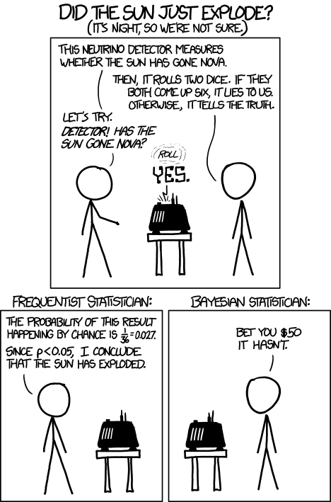
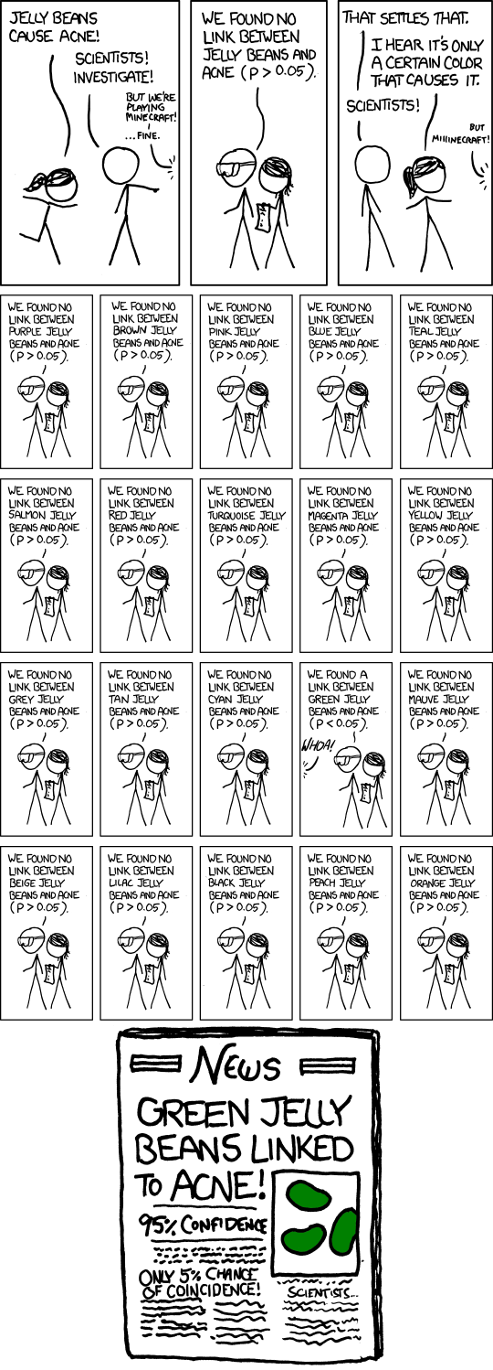
Peeking is the practice of inspecting results before the planned sample size is reached and stopping early if the numbers look good. It is what invalidates frequentist tests when p-values are checked repeatedly mid-experiment — the false positive rate inflates because you are effectively running multiple tests and keeping the best result. The same logic applies to the Bayesian posterior.

Run enough tests, check often enough, and green jelly beans will cause acne. The Bayesian equivalent: check the posterior enough times and your rewards program will appear to work. The AV subsidy line item does not care which framework licensed your false positive.

If you evaluate $p_\text{wrong} < \epsilon$ continuously and stop the moment it dips below threshold, you have not run the experiment described by the formula above. You have run something different, with different — and worse — statistical properties. The Bayesian framing does not make this problem disappear. It reframes it. The stopping rule is still a rule, and it must be respected as such.

The Deeper Point

Now consider what happens when you align the frequentist and Bayesian parameters. Under a non-informative prior and Gaussian approximation:

$$\left[ \Phi^{-1}(1-\epsilon) \right]^2 = \left( z_{1-\alpha/2} + z_{1-\beta} \right)^2$$

The two formulas are identical. After one round of experimentation, you can always set $\hat{\theta}_A = \theta_A$ and the sample sizes converge exactly. The Bayesian framework is not buying you a smaller experiment — it is buying you a different interpretation of the same data collected over the same period, subsidising the same number of AV rides.

The cost of the rewards program does not go down because you chose a different statistical paradigm. The experiment still needs to run for exactly as long as the sample size demands, the rides still need to be subsidised for the duration of it, and the rewards program still costs the same amount of money regardless of what you call the statistical framework governing your decision.

If there is a genuine desire to reduce experiment duration, the honest levers are: a larger expected effect size (better rewards design), higher tolerance for error ($\epsilon$ or $\alpha$), or accepting lower power. Switching from frequentist to Bayesian and calling it done is not one of them.

Beyond Photons: Passive Acoustic Sensing for Autonomous Vehicles

2026-03-07T00:00:00.000Z

Introduction

In autonomous driving, perception systems typically rely on photons i.e. cameras, lidar, and radar. But what if we could also listen to the environment, capturing sound cues that are invisible to traditional vision-based sensors?

There are many intuitively appealing use cases where an additional sensing modality could enhance awareness of the surroundings. Acoustic sensing itself is not new in automotive systems. For example, ultrasonic sensors have long been used for short-range applications such as parking assistance. Extending this idea to environmental sound sensing—allowing a vehicle to effectively hear its surroundings—has been explored by organizations such as the Fraunhofer Institute and Renesas Electronics. At CVPR ‘23 we had the Princeton Computational Image lab create 2D “images” using beamforming (more on this later) from passive acoustic listening and fused this with RGB camera data.

While the Princeton paper was highly influential to this work, our client was interested in passing certain scenarios only without overly relying on (or expending energy on) a highly complex multi-dimensional sensor modality. In this post we explore several motivations for adding a simpler version of passive acoustic sensing to the autonomous vehicle sensor stack.

Sneak Peek of our solution: Flashing red/cyan vehicle is emitting sound

Why consider acoustic sensing?

Obstructed-view scenarios are increasingly emphasized in safety standards such as Euro NACP. Detecting hazards before they become visible is critical for improving safety metrics.
With the rise of autonomous systems in defense and security applications, additional sensing modalities may provide a differentiator when competing for contracts.
Sound does not require line-of-sight (LoS). Important events such as children playing in the street, emergency vehicle sirens, or approaching traffic can be detected even when visually occluded.
Sound is a natural communication modality for humans, and could provide a mechanism for richer interaction between the environment and the ego vehicle.
Acoustic signals can intrinsically provide directional information (heading), which can improve situational awareness metrics such as MAPH (Mean Average Precision with Heading).
Beamforming+RGB outperforms RGB alone in challenging occluded scenarios

Key disadvantages

Acoustic sensing also introduces several challenges:

Passive acoustic systems typically provide Angle-of-Arrival (AoA) information but not reliable distance estimates.
Performance can degrade due to vehicle noise, wind noise, and environmental interference.

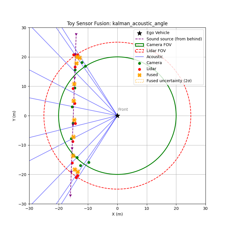
Toy Example: Acoustic Direction Improves Early Detection

To illustrate the value of acoustic sensing, consider a simple scenario:

An emergency vehicle approaches from the bottom-right relative to the ego vehicle.
Acoustic sensing estimates the direction of arrival using TDOA between microphones, but cannot determine distance.
Camera and lidar only detect the vehicle once it enters their field of view.

In the simulation, the vehicle moves toward the ego vehicle. The acoustic system continuously estimates a sextant, or directional sector, while the camera and lidar begin detecting the vehicle only after it enters their sensing range.

This allows the fusion system to gain early directional awareness, giving planning systems a chance to anticipate the approaching vehicle before visual confirmation. Even though the acoustic angle estimate is noisy, it provides information beyond the field of view of both camera and lidar. After fusing with lidar and camera data, the system produces more accurate position estimates.

Context

The work described here was originally developed at Reality AI, which was later acquired by Renesas Electronics to explore the commercial feasibility of passive acoustic sensing in automotive systems. My role focused on scaling the solution and validating it across different environments.

We conducted experiments using simulated emergency sirens in multiple environments, including:

controlled warehouse setups
busy urban streets
open environments with realistic traffic noise

We also collaborated with external partners to collect additional datasets and explore multi-sensor fusion approaches.

In this article, I will explore PAMVON (Passive Acoustic Monitoring for Vehicles and Objects)—a system that uses microphone arrays, signal processing, and machine learning to detect and localize important acoustic events in the driving environment.

We conducted experiments using simulated emergency sirens in multiple environments, including:

controlled warehouse setups
busy urban streets
open environments with realistic traffic noise

We also collaborated with external partners to collect additional datasets and explore multi-sensor fusion approaches.

Passive Acoustic Monitoring (PAM)

Passive Acoustic Monitoring (PAM) detects environmental sounds without emitting signals. Instead, the system passively listens for events in the surrounding environment such as emergency vehicle sirens, horns, tire skids, engine noise, drones or machinery, and even children playing in the street.

The key advantage of this approach is that sound does not require line-of-sight. Important cues can be detected even when they are visually occluded, in low-light conditions, or in adverse weather. This makes acoustic sensing particularly attractive for early warning scenarios, such as an approaching ambulance that has not yet entered the field of view of the vehicle’s cameras or lidar.

Recent developments in multimodal large language models also change how one might think about acoustic perception. Rather than requiring a rigid classifier that assigns each sound to a predefined category, modern multimodal systems can reason over audio signals more flexibly and incorporate them into a broader contextual understanding of the scene. In practice this means the acoustic signal can act less as a strict classification task and more as an additional stream of environmental information that the perception system can interpret alongside vision and other sensor modalities.

Microphone Arrays and Beamforming

Sound (like light) travels in a straight line and therefore we need at least 4 microphones to provide an accurate estimate of the angle of arrival of the sound wave.
A single microphone provides limited spatial information. To estimate where a sound originates, passive acoustic monitoring systems typically use small arrays of microphones. By observing the time differences between when a signal reaches each microphone, the system can estimate the direction of arrival of the sound source. Arrays also make it possible to improve signal quality by combining signals from multiple sensors.

In practice this enables several useful capabilities. The system can estimate the direction of arrival of a sound, approximate the location of the source under certain assumptions, and improve the signal-to-noise ratio by combining measurements across the array.

Beamforming is the signal processing technique that makes this possible. The idea is simple: signals arriving from a particular direction reach each microphone at slightly different times. By applying the appropriate delays and summing the signals together, the array reinforces sounds from the desired direction while suppressing sounds from other directions.

The microphone array can be visualized like this:


Mic1 ----------- Mic2
   \               /
    \             /
     \           /
       ( sound )
         source
     /           \
    /             \
   /               \
Mic3 ----------- Mic4

In practice the system estimates the relative delay between microphones using cross-correlation. When a sound arrives at the array, it reaches each microphone at slightly different times. By computing the cross-correlation between pairs of microphone signals, the system can estimate the time difference of arrival between them.

These time differences constrain the direction from which the sound could have originated. With multiple microphone pairs, the system can estimate a consistent direction of arrival for the source.

Once the delays are known, the array can also combine the microphone signals in a way that reinforces sounds coming from that direction while suppressing others. In effect, the array behaves like a steerable listening sensor that can focus on different parts of the acoustic scene.

Angle of Arrival (AoA) Estimation via Cross-Correlation

In a microphone array, a sound source reaches each microphone at slightly different times. By comparing these signals, the system can estimate the relative delay between them. A common way to do this is through cross-correlation, which measures how similar two signals are as one is shifted in time relative to the other.

For two microphone signals $x_1(t)$ and $x_2(t)$, the cross-correlation can be written as

$$R_{12}(\tau) = \int x_1(t) \, x_2(t+\tau) \, dt$$

The time shift $\tau$ that maximizes this correlation corresponds to the time difference of arrival between the two microphones:

$$\tau_{\text{max}} = \arg\max_\tau R_{12}(\tau)$$

If the microphones are separated by a distance $d$, this delay can be converted into an estimate of the angle of arrival:

$$\theta = \arcsin\left(\frac{c \cdot \tau_{\text{max}}}{d}\right)$$

where $c$ is the speed of sound.

In real environments, reflections and background noise can make the correlation peak less reliable. A commonly used approach to improve robustness is generalized cross-correlation with phase transform (GCC-PHAT). This method emphasizes phase information in the frequency domain and reduces the influence of signal magnitude differences:

$$R_{12}(\tau) = \mathcal{F}^{-1}\{\frac{X_1(f) X_2^(f)}{|X_1(f) X_2^*(f)|}\}$$

Here $X_1(f)$ and $X_2(f)$ are the Fourier transforms of the microphone signals. The peak of $R_{12}(\tau)$ provides a stable estimate of the arrival delay, which can then be used to infer the direction of the sound source.

Signal Processing Pipeline

Passive acoustic monitoring typically follows a structured processing pipeline:

Preprocessing: The raw microphone signals are filtered to remove irrelevant frequency bands, and gain normalization ensures consistent amplitude levels across microphones.
Time-frequency analysis: Signals are converted into spectrograms using the Short-Time Fourier Transform (STFT), revealing how frequency content evolves over time.
Beamforming: Directional enhancement techniques, such as delay-and-sum or cross-correlation-based beamforming, focus on sounds from specific directions while suppressing noise and interference.
Event detection: Open-source neural networks, including VGGish, convolutional-recurrent networks (CRNNs), and transformers, analyze the spectrograms to detect and classify events such as sirens, horns, or tire skids.
Localization: Time Difference of Arrival (TDOA) estimates, often computed using GCC-PHAT cross-correlation, are combined across microphone pairs to infer the direction of incoming sounds and, in some cases, approximate source locations.

This pipeline allows the system to transform raw audio into actionable information for autonomous vehicle perception, providing early warning of hazards even when they are outside the line of sight of cameras or lidar.

Acoustic Sensor Data Representation

In a generalized form, data from a passive acoustic monitoring array can be represented as a tuple capturing the relevant information for fusion:

$$\displaystyle z_{\mathrm{ac}} = (\theta, \sigma_\theta, c, f, t, p_{\mathrm{ego}})$$

Where:

$\theta$: Estimated angle of arrival (AoA) of the sound, typically computed using TDOA and cross-correlation (GCC-PHAT).
$\sigma_\theta$: Uncertainty of the angle estimate, reflecting noise, reverberation, or low SNR.
$c$: Sound class probability vector produced by the ML model. The classes correspond to ambulance, police, and other unknown loud sounds. For example, $c = [0.7, 0.2, 0.1]$
$f$: Frequency-domain features, such as Mel spectrogram or STFT frame, optionally used for downstream ML fusion.
$t$: Timestamp of the measurement, to allow temporal alignment with other sensors.
$\mathbf{p}_{\text{ego}}$: Pose of the ego vehicle when the measurement was captured, typically $(x, y, \psi)$ in 2D or 3D coordinates.

This representation allows the acoustic signal to integrate easily into perception and fusion pipelines:

$\theta$ provides a directional prior for early detection.
$c$ informs semantic understanding of the source.
$\sigma_\theta$ can be used in probabilistic fusion (e.g., weighted averaging, Kalman updates).
$f$ allows future retraining or fine-tuning of ML models.
$t$ and $\mathbf{p}_{\text{ego}}$ allow projection into bird’s-eye view (BEV) maps or occupancy grids alongside camera and lidar data.

For an array of $N$ microphones, the raw signals can also be stored as:

$$\mathbf{X}_{\text{raw}} = [x_1(t), x_2(t), \dots, x_N(t)]$$

These raw signals are processed into the generalized form above, providing a compact yet rich representation for sensor fusion.

Simple ID-Based Matching

Before exploring a more technical late fusion approach, we first evaluated a simpler strategy based on ID matching. In this setup, acoustic detections were associated directly with annotated object identities in the dataset.

The acoustic classifier produced class probabilities for events such as ambulance sirens, police sirens, or other loud sounds. When the classifier detected a high probability ambulance siren, we matched that event to the corresponding object detection annotation in the scene. In practice this meant associating the acoustic event with the object ID labeled as an emergency vehicle in the perception dataset.

One challenge is that the acoustic detector often produces a directional estimate much earlier than the moment when the vehicle becomes visible and is annotated by the vision system. The acoustic pipeline provides an angle of arrival $\theta$, but not a direct range estimate. To place this information in the BEV representation, we projected the acoustic bearing into the map by creating an artificial point along the direction of arrival at a fixed distance $d$ from the ego vehicle. The distance was chosen to be larger than the field of view of the camera and lidar sensors so that the acoustic signal could represent a potential source outside the current perception range.

This artificial point can be written as

$$p_{ac} =\begin{bmatrix}x_{ego} \\y_{ego}\end{bmatrix}+d\begin{bmatrix}\cos \theta \\\sin \theta\end{bmatrix}$$

where $(x_{ego}, y_{ego})$ is the position of the ego vehicle in BEV coordinates. As the vehicle approaches and eventually enters the sensor field of view, the projected acoustic point becomes spatially consistent with the detected object.

This approach relies on the object detection pipeline already identifying vehicles and assigning consistent IDs across frames. The acoustic system then acts as an additional signal that confirms the presence of a specific type of vehicle.

Although simple, this method is surprisingly effective. The acoustic cue provides early detection of emergency vehicles, while the vision system provides precise localization and tracking. By linking the acoustic classification to existing object IDs, the system can quickly identify which tracked object is likely producing the sound.

This ID-based matching served as a useful baseline before implementing a more general late fusion approach using probabilistic tracking and bearing measurements.

Late Fusion with an Existing BEV Pipeline

While the ID-based matching approach provided a strong baseline, it relies on the object already being detected and assigned an identity by the perception pipeline. In many cases the acoustic signal appears earlier, before the vehicle enters the field of view of the cameras or lidar. To make better use of this early directional information, we extended the system using a more formal late fusion approach.

In this setup, acoustic sensing was integrated on top of an existing lidar and camera perception stack. The vision and lidar pipeline already produced tracked objects in bird’s-eye view (BEV), including estimates of position, velocity, and uncertainty. The acoustic sensor then contributed an additional bearing measurement, which could be incorporated into the tracking framework to refine object estimates and improve situational awareness.

After lidar and camera fusion, each tracked object is represented by a state vector

$$\mathbf{x} =\begin{bmatrix}x \\y \\v_x \\ v_y\end{bmatrix}$$

where $(x,y)$ represents the position of the object in BEV coordinates and $(v_x, v_y)$ represents the velocity components. The tracker also maintains a covariance matrix

$$\mathbf{P}$$

which represents the uncertainty of the state estimate.

The acoustic system produces a bearing measurement corresponding to the direction of arrival of the sound:

$$z_{ac} = \theta$$

where $\theta$ is the estimated angle of arrival relative to the ego vehicle.

If the ego vehicle is located at position $(x_e, y_e)$, the predicted bearing of a tracked object can be written as

$$h(\mathbf{x}) =\arctan2(y - y_e, \; x - x_e)$$

This function maps the tracked object position into the expected acoustic measurement.

The difference between the observed bearing and the predicted bearing is the innovation:

$$\mathbf{y} = z_{ac} - h(\mathbf{x})$$

Because the measurement model is nonlinear, we linearize it using the Jacobian

$$\mathbf{H} =\begin{bmatrix}\frac{\partial h}{\partial x} &\frac{\partial h}{\partial y} &0 &0\end{bmatrix}$$

For the bearing function this yields

$$\frac{\partial h}{\partial x} = -\frac{y - y_e}{(x-x_e)^2 + (y-y_e)^2}$$$$\frac{\partial h}{\partial y} = \frac{x - x_e}{(x-x_e)^2 + (y-y_e)^2}$$

Given acoustic measurement noise $R_{ac}$, the Kalman gain can then be computed as

$$\mathbf{K} =\mathbf{P} \mathbf{H}^T(\mathbf{H} \mathbf{P} \mathbf{H}^T + R_{ac})^{-1}$$

The updated state estimate becomes

$$\mathbf{x}_{new} =\mathbf{x} + \mathbf{K}\mathbf{y}$$

and the covariance is updated as

$$\mathbf{P}_{new} = (I - \mathbf{K}\mathbf{H})\mathbf{P}$$

Since the acoustic sensor only provides directional information, this update primarily reduces uncertainty perpendicular to the acoustic ray while leaving uncertainty along the ray largely unchanged. In practice, this allows acoustic measurements to improve the tracking of objects detected by lidar and camera without requiring modifications to the existing perception pipeline.

Final Output

The final output of the system is represented in Bird’s-Eye View (BEV) space. The acoustic information can be projected into this space using either of the two methods discussed earlier.

In the example scene below, the ego vehicle drives past a stationary car that is simulated to emit an emergency vehicle siren. The figure illustrates how the acoustic signal integrates with the rest of the perception stack.

On the left, we show the acoustic output tagged with an object ID from the real-time object detection system provided by the customer (likely based on a model such as YOLO).

In the centre, we show the BEV representation, where the estimated angle of arrival (AoA) from the microphone array is plotted as a ray originating from the ego vehicle. Because the clip is only six seconds long, the visualization shows a ray pointing in the direction of the detected emergency vehicle sound from the start of the sequence. In this case, the microphones detect the siren before the object enters the field of view of either the camera or the lidar.

Once the vision-based detector identifies the vehicle, the AoA estimate can be associated with that object, with small corrections applied if necessary to account for sensor alignment or localisation error.

On the right, we show the lidar point cloud for the same scene. In this example, the acoustic output is not annotated in the lidar view, although such a visualization is also possible.

Camera: Flashing red/cyan vehicle is emitting sound

BEV: Acoustic AoA Plotted

LiDAR

Implementation Considerations

The passive acoustic monitoring pipeline can be implemented efficiently on embedded automotive hardware. In our implementation, the audio processing pipeline, machine learning inference, and angle of arrival estimation were designed to run on a single MCU core. This includes signal preprocessing, spectrogram generation, neural network inference, and cross-correlation based localization.

The system was implemented on Renesas automotive controllers, specifically the RH850 microcontroller family. Audio input processing, AI target detection, and angle of arrival estimation ran on a single RH850 core alongside the A2B audio stack. In this configuration the full acoustic pipeline occupied roughly 300 KB of code space, even while running in a debug configuration and without aggressive optimization.

This relatively small footprint makes it feasible to deploy acoustic sensing alongside other perception tasks without requiring specialized hardware acceleration. On RH850 devices, significant CPU, flash, and RAM resources remain available for additional vehicle functions.

Microphone array configurations can also be adapted depending on coverage requirements. A four-microphone array provides approximately 180 degrees of coverage, while an eight-microphone configuration enables full 360 degree sensing around the vehicle.

In practice, the computational requirements depend on the complexity of the processing pipeline. Efficient PAM processing can run entirely on automotive-grade microcontrollers such as the RH850. Larger microphone arrays or more complex neural networks may benefit from more powerful automotive SoCs such as the Renesas R-Car platform. Regardless of the hardware platform, maintaining real-time processing is critical so that acoustic events can be incorporated into the perception pipeline with minimal latency.


   Microphone Array
(4 or 8 digital microphones)
         │
         │
         ▼
 +------------------+
 |   A2B Audio Bus  |
 | (Automotive Audio|
 |   Backbone)      |
 +------------------+
         │
         │
         ▼
 +----------------------+
 |   RH850 MCU          |
 |----------------------|
 |  Audio Preprocessing |
 |  STFT / Spectrogram  |
 |  VGGish Inference    |
 |  GCC-PHAT (TDOA)     |
 |  AoA Estimation      |
 +----------------------+
         │
         │
         ▼
 +----------------------+
 |  Acoustic Detection  |
 |  θ (bearing)         |
 |  class probabilities |
 +----------------------+
         │
         │
         ▼
 +----------------------+
 |   BEV Fusion Layer   |
 | (Camera + Lidar +    |
 |    Acoustic)         |
 +----------------------+
         │
         ▼
 +----------------------+
 |  Tracking / Planning |
 +----------------------+

Conclusion

Passive acoustic monitoring has shown significant potential but has not yet become standard in autonomous vehicle perception stacks. There are several challenges that limit its adoption:

Ambient noise and signal variability – urban environments are full of sounds that can mask sirens, horns, and other important cues.
Environmental acoustic complexity – reflections, occlusions, and vibrations from the vehicle itself make accurate localization difficult.
Automotive qualification and safety standards – microphones and processing hardware must meet rigorous requirements such as ISO 26262 and AEC-Q100, and survive extreme temperatures and vibrations.
Limited generalization of machine learning models – systems that perform well in controlled tests can struggle on highways, in multi-siren urban settings, or with unusual sound events.
No regulatory requirement – without a mandate from safety standards or OEMs, there is little commercial incentive to integrate acoustic sensing into production vehicles.

Despite these obstacles, acoustic sensing can still provide value when used as a complementary modality. Integrating sound cues through late fusion on top of camera and lidar tracks allows early warnings of approaching emergency vehicles or other hazards, even before they enter the field of view. In this way, the acoustic signal reinforces and augments traditional sensors, enhancing situational awareness without requiring a full redesign of the perception stack. Performance improvements were observed in EuroNACP obstructed view testing scenarios, demonstrating the practical benefit of including an acoustic modality in complex urban environments.

References

Renesas Electronics. Seeing Sound: AI-Based Detection of Participants in Automotive Environment Using Passive Audio. White Paper.
https://www.renesas.com/en/document/whp/seeing-sound-ai-based-detection-participants-automotive-environment-passive-audio?r=1626806
Princeton University Light + Sound Interaction Lab. Seeing with Sound.
https://light.princeton.edu/publication/seeingwithsound/

From Bits to Clocks: A Visual Intuition for the Quantum Fourier Transform

2026-02-28T00:00:00.000Z

Introduction

Sometimes it does seem like my blog is just increasingly complex applications of the Fourier Transform. In the previous post we applied the Fourier Transform to graphs, drawing connections between frequency (which is the usual Fourier transform) and properties of the graph. There is yet another interesting, if abstract, application of the Fourier transform that is used in Quantum computers. Somewhat surprisingly, it is called the “Quantum Fourier Transform”. More specifically, we will study how the Fourier Transform appears as a unitary linear operator acting on quantum states.

At the end of the day this is all just linear algebra, requiring no knowledge of actual quantum physics. Because the Quantum Fourier Transform can be somewhat mathematically abstract and also because the Fourier Transform is so easily visualized as a decomposition into various sines and cosines, I thought of coming up with a similar visualization for the Quantum Fourier Transform case (spoiler: it involves clocks).

Motivation

Before discussing in detail what the QFT is mathematically, it is useful to recap what the Fourier transform is in general. The Fourier transform is a way of transforming information from one domain to another domain. Why? Because certain operations become simpler in the transformed domain. For example, in classical signal processing, convolution of a signal (the mathematical definition of filtering) in the time domain corresponds to simple multiplication in the frequency domain.

In the graph setting, we saw that potentially complex behaviors in the edge-node representation of the graph were far more mathematically tractable when looking at the “frequency” equivalent of the graph. Eigenvectors of the graph Laplacian isolate modes of variation: low-frequency components capture global structure, while high-frequency components capture local fluctuations.

Similarly, for the Quantum Fourier Transform, we move from a bit representation of a number to a cyclical or phase representation. In the computational basis, information is stored as binary digits, essentially a sequence of ON/OFF switches taking values in $\{0,1\}$.

In this form, the data is linear and rigid. Any underlying periodic structure is hidden inside the positional encoding. Phases, however, live on the circle and are inherently cyclical. If we want to detect periodicity or modular structure, it is more natural to encode information as rotations rather than switches.

The QFT therefore plays the same conceptual role as the classical Fourier transform: it changes coordinates to a representation in which the problem’s hidden structure becomes easier to manipulate.

I might do a post later on why this is true on so many different problems. But it is not true for some problems such as when you need convolution to learn a local filter.

Useful Intuition

One of the reasons the Fourier transform in its simplest form is so
interesting is that it is so visual. In this blog post I will try to provide a nice visual explanation for
the QFT. Essentially we want to draw a connection between the binary
representation of a number and the cyclical nature of the QFT.
Fortunately, there is a nice visual representation for a binary
representation of a number on a computer, called a qubit. This
representation of a number is called a qubit.

A Useful Visualization

Signaling, Skills, and Intellectual Health in the Age of AI: Thoughts from UChicago Career Conference 2026

2026-02-20T00:00:00.000Z

Introduction

I was recently invited back to the MA department at UChicago for a career conference. Sitting there, listening and speaking, I found myself asking a rather uncomfortable question:

How much of what we value in education is pure signaling? Is this still true in the age of AI?

It is perhaps an opportune moment to recap the signaling model of education. In labour markets with asymmetric information, employers cannot directly observe ability. In Michael Spence’s signaling model, education does not necessarily increase productivity; instead, it separates high-ability individuals from others because it is less costly for them to acquire. In this paradigm, education serves as a “signal” of ability.

I think AI has changed this status quo because the cost of acquiring education has reduced to the point that there is no cost differential between high-ability and low-ability individuals for a large number of courses. To be more specific, the cost of sending a signal of education is reduced to the point of being indistinguishable between both groups. The cost of actually educating oneself is likely still lower for high-ability individuals, it’s just that sending this signal is easier.

This essay is intended to answer some of the questions that I recieved at the conference, some of which are outlined below,

But what does “actually” educating oneself really mean?
What does it look like? Which classes should I take?
What should be the emphasis of my self-study?
How do I position myself best for the job market?

Beyond The Signal: So What Should I Study?

In the old (read: pre-AI) world where education was largely signaling, I think taking classes that superficially but with high probability signaled education, such as cloud skills, basic Python programming, and machine learning applications, were good enough. But in the new world, the cost of acquiring these skills is zero. Thus high-ability individuals need to seek out higher difficulty tasks that are relatively lower cost for them to acquire in order to send a strong signal. Mathematical maturity, comfort with abstraction, and disciplined reasoning are not signals in themselves; they are capabilities that affect what you can build, debug, or invent.

Thus class choices should reflect these core values:

Mathematical courses that emphasize the core mathematics that make up machine learning, such as linear algebra and differential equations
Looking under the hood of machine learning, focusing on the mathematical fundamentals of machine learning
Social sciences courses that challenge your world view and force you to think about what the world should look like (more on this below)

Good Intellectual Health

More important than ever, and not specific to tech jobs but just life in general, is maintaining good intellectual health.

Reading books both in your field and outside of it is now more important than perhaps in the world before AI. Using AI increases one’s distance from one’s self. One’s ideas and one’s thoughts are now further than ever from one’s own experience. Reading books and writing reduces this distance. Since idea generation and critical thinking depend so heavily not only on the final output but also on the process by which one reaches it, exercising this muscle is now more important than ever.

Maintaining good intellectual health, however, is almost entirely self-policed. There are very few reliable ways to monitor how much AI shapes one’s own work. What usually starts as submitting homework in a rush can escalate to generating entire essays using AI, the slope is truly slippery. One cannot afford to replace the cognitive effort that builds depth, originality, and judgment. Only you can decide if the level of AI use hampers your intellectual health, and only you can feel its effects.

The sciences are exceptionally good at helping us understand what the world is. As a result, advice about improving technical skills tends to be prescriptive and measurable. The social sciences operate differently. They help us think about what the world should look like. They force us to articulate assumptions about behaviour, incentives, norms, and institutions. The process of forming a view about what the world ought to be is central to intellectual health. It requires reflection, judgment, and an awareness of values, not just optimisation. Admittedly, this is difficult advice to give at a career conference for students focused purely on technical roles. The impact of studying sociology, psychology, or economics is harder to measure in a tech performance review. It doesn’t map cleanly onto a skills matrix. But it is no less important for that reason. The social sciences implicitly construct world models. Whether in sociology, psychology, or economics, they offer structured ways of thinking about how systems of people behave. That kind of world-building is essential for understanding where highly parameterised models, such as those produced in machine learning, actually live. Models do not operate in a vacuum; they operate within social and economic systems.

This becomes even clearer in business contexts. Firms operate with explicit views of what the world should look like, in terms of acquisition, churn, retention, revenue. Machine learning systems are deployed inside those normative visions. I admit there is something slightly distasteful about motivating the social sciences purely in terms of churn or revenue. It feels almost sacrilegious. But in practice, those incentives shape the environments in which technical systems are built. And if that were not the case, the audience at a career conference might be asking very different questions, comrade.

TL;DR;

The “sticker” value of UChicago’s education has held steady relative to other similar institutions. It might even have appreciated slightly. However, the absolute “sticker” value of education as a signal of ability in top schools (and indeed everywhere else) has gone down. Thus the onus is now on students to take courses that more appropriately signal their ability, not just in purely technical terms (such as mathematics, physics, machine learning) but also in critical thinking terms (such as expertise in the social sciences). The days of superficial knowledge that use model.fit(X) are over.

The UChicago brand will likely hold its value for years to come but it is not going to be enough. Even though the bar to have superficial knowledge is lowered thus muddying the difference between high and low skill individuals, the bar to have truly fundamental understanding of the sciences including (and perhaps especially) the social sciences is has never been higher.

On Murakami

2026-01-15T00:00:00.000Z

Introduction

I did not spend my twenties reading Murakami, when it was all the vogue. Now, having read three works of his, I feel an upswell of opinions on his work and writing. We will explore some of the themes of Murakami as well as the cultural symbol that he has become. He was the kind of writer you are almost supposed to like as a young man.

Murakami seemed like the sort of writer you are supposed to like, especially in your twenties. Sadly, my twenties flew by rather quickly without so much as a glance at a Murakami novel. And there were several — part of Murakami’s appeal is how prolific he is across a variety of genres. Now in my, arguably still early, thirties I have read three novels of his: Kafka on the Shore, First Person Singular, and The Wind-Up Bird Chronicle. While my views on Murakami remain lukewarm at best, his writing certainly inspires deeper engagement with broader themes in society.

Writing

The English literary tradition has always been deeply rooted in the beauty of language; it is almost as if the words carrying the story must match the beauty of the story itself. The result can be complex, layered prose that oftentimes outlasts the literary work itself. Very often from the opening lines themselves, the classics sought to set the stage with beautiful prose.

“Call me Ishmael…”, “It was the best of times, it was the worst of times…”

Compare this with Murakami, whose writing proceeds forth incessantly in its banality. The words easily slide off the page as if narrated by a friend over the telephone. The words do not linger; they hurry off the page carrying their message with great efficacy. He does not, however, use this efficiency to drive more of the plot forward, choosing instead to match the banality of his prose with descriptions of the banalities of the human condition — eating, sleeping, and listening to music. It seems as if Murakami rejects the aestheticism of both the prose and the story. One cannot imagine Dickens devoting a paragraph to what the main character ate for breakfast.

One should not leave with the impression that the resulting writing is uninspired or insipid. On the contrary, the effect of his writing is a highly atmospheric narrative style that attenuates his trademark surrealistic elements. The banalities serve to obscure or highlight the passage of time, a critical element of his surrealistic themes. The reader is drawn into a different world, and very often drawn into a different supernatural world within that world.

A long-standing critique of English literature prior to Murakami was that it was almost inaccessible to people learning English for the first time. In my eyes this was largely a consequence of English speakers dominating English writing, whereas Murakami does not speak English as his first language. Nothing exemplifies this more than the fact that Murakami came upon his extraordinarily simple writing style by simply translating his English prose to Japanese and then back, thus losing all but its most essential elements. Literary essentialism, some (this author) would call it.

Nothing is happening here. The shrine stands. The snow falls. And yet — this is precisely the kind of scene Murakami would spend three pages on, and you would read every word of it. The atmosphere is the point; the banality is the vehicle. This is the closest image I can find to what it actually feels like to read him.

Eastern Storytelling

There is a tension between Eastern and Western storytelling, and this tension is apparent even in the differences in children’s stories. In Grimm’s fairy tales, for example, we have a clearly defined protagonist who must weather the odds, defeat the antagonist, and eventually prevails. In Eastern storytelling the beauty of the story is much more important than what the story means. Consider The Crane Wife, a well-known Japanese children’s story. A crane transforms into a beautiful woman; this beautiful woman proposes to a poor fisherman. The fisherman agrees, but the woman imposes one condition: he can never look at her when she is weeping. One day the fisherman looks at her while she weeps; he sees that she is a white crane. He leaves her. The story ends, rather abruptly. This ending is rather distressing, especially to Western audiences. Why does the story end? The ending is so sad — how can it end yet? What does this all mean? Beauty, I suppose, is the key to this difference. This is a beautiful story and the sadness is beautiful.

The moon reflects on the water. The islands sit in the dark. No story. No explanation. No moral. And it does not matter — the image is enough. This is what Eastern aesthetic beauty looks like when it works. Murakami is reaching for something like this. I am not always sure he grasps it.

I have the same visceral reaction to Murakami’s stories. I find myself asking at the end of every book:

But what does this all mean?

While I recognize that this cultural difference is at the heart of why people react negatively to Murakami’s writing, I find it hard to reconcile with the fact that Murakami’s writing forces you to do one of two things.

The first is to take the story literally. This involves taking every supernatural act, every bizarre event as literal and believing it. This is not hard — we do this to some degree with all works of fiction, from Tolkien to Kafka. We are (I am) willing to suspend disbelief. However, the stories take themselves seriously. In The Metamorphosis, while we are never offered an explanation for why Samsa is a monstrous insect, the reactions to him and his reactions to himself treat his metamorphosis as real. The story takes itself seriously and reconciles the apparent inexplicability of the metamorphosis as given. This is not the effect that Murakami’s writing has on me. His writing weakly evokes bizarre situations such as the insect; however, there are a great many such situations. The immoderation in the supernatural and the bizarre requires a much higher degree of suspension of disbelief, which makes it much harder for the reactions of other characters to be believable. It reminds me of the famous Christopher Nolan quote:

“It does not matter how believable the story is to you; the story must be believable to itself and its characters.”

It is this inviolable rule that is broken multiple times.

The second is to take the story as some kind of metaphor. Again, Kafka’s writing has this effect as well — we can think of the insect-like transformation of Gregor Samsa as a kind of moral corruption, stagnation, or emasculation. However, because Murakami uses characters, bizarre events, and other supernatural motifs so liberally, it is difficult for the metaphor to retain any coherent narrative structure, let alone a consistent representation of something else.

In both cases, it seems as if Murakami is willing to sacrifice coherence and linguistic beauty for some kind of narrative aesthetic. To me this sacrifice was not worth it, since there are far too many characters and motifs that seem to exist solely to move the plot along. Far too many characters are sacrificed on this imagined altar of aesthetic beauty. My objection does not arise out of a sense of wellbeing for these characters, but rather that they seem rather superficial — which leads naturally to my next criticism.

Superficiality

The main characters in Murakami’s books can be disappointingly without agency. They can seem as if they are carried away by the wave of the narrative. This matches Murakami’s style in his own words: he creates the characters first and then places them in a story. Almost like a simulation — this makes the storytelling easy.

Again, this could be the difference between Eastern and Western protagonists. I do not agree with this, however. I think Murakami’s characters are quite American in a modern way. The protagonist is like the main character in a pop culture film — hidden away, not a part of society. But then society needs him, or something happens to him, and he must act in the midst of it. In some strange way this superficiality matches the aesthetic of Murakami’s writing. In some ways, I consider Murakami to be a modern American author, as much as Paul Auster. To Murakami’s credit, I suspect this imitation might not be entirely unintentional. This imitation evokes the adoption of Western individualism by Japanese society — fairly thin, and without the corresponding import of Christian ethics. Murakami laments the lack of family connections in Japanese society.

Similarly, supporting characters exist only as reflections of the main character. In all the books that I read, I was not able to identify one single character that had anything remotely resembling a personality. Murakami writes a superficial main character and every other character exists to reflect that character back to himself. Bizarrely, Murakami’s novels feel two-dimensional — you are drawn into an atmospheric but ultimately flat world. Some things feel real, but the lack of dimension is apparent. It has to be said that this is appealing to some; others describe this as “dreamy”, “vague”, and “beautifully foggy”. It is likely that this flaw uniquely penetrates my intellectual armor more so than others.

I have many issues with the way women are written in Murakami’s novels. I will leave it at that.

Japanese Psyche

It is somewhat contradictory that Murakami is surprisingly modern, and almost comes across as an American writer in some sense. Yet the questions his books raise about Japanese identity — individualism imported wholesale from the West, the erosion of family and community — are distinctly Japanese concerns, and they are the more interesting for it.

Conclusion

I find myself, having now read three of his novels, in the rather uncomfortable position of a reluctant critic. Murakami is undeniably significant. He has done more for the global reach of Japanese literature than perhaps any other living author, and his ability to inhabit the borderlands between the real and the supernatural is a genuine literary achievement. His cultural impact is not nothing, as the young person in every bookshop clutching a copy of Norwegian Wood will attest.

But the books themselves leave me cold — not in a sterile sense. They are atmospheric, readable, and at times deeply evocative. I always emerge from them, however, without the feeling of having had a meaningful encounter with another human mind. The characters drift, the plots dissolve, and one is left with that same persistent question.

But what does this all mean?

I suspect that for his devoted readers, the answer is in the question itself. The asking is the point. The fog is the destination. I remain unconvinced, but I respect the fog.

Murakami’s world looks something like this — solid enough to walk through, obscured enough to never quite see the edges of. The fog does not owe you an explanation. I have made my peace with this, though not enough to enjoy it.

Telegraph Hill and the Coastline Paradox: Measuring a City in Fractional Dimensions

2025-12-16T00:00:00.000Z

Introduction

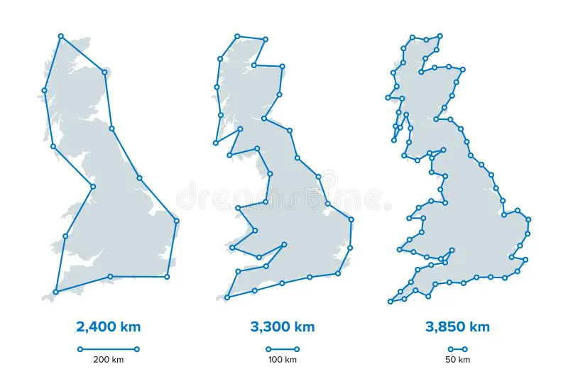
If you’ve ever come across the coastline paradox, you’ve probably seen the classic (and somewhat overused) image of the coastline of Britain. Recently, a friend asked me a question that felt like the 3D analogue of this paradox: What is the surface area of a city? More specifically, does a very hilly city have more surface area than a relatively flat one?

The answer, as it turns out, is more complicated than it first appears. My initial instinct was to treat this as the 3D version of the coastline paradox, and that idea sent me down a rabbit hole—one whose key insights form the basis of this blog post.
Complete follow along notebook can be found here.

Here’s how the post is structured:

Visualizing the 2D coastline paradox using the Koch curve, a well-known fractal curve.
Extending this to the 3D case by visualizing the surface area paradox with a fractal terrain.
Applying these ideas to real-world GIS data to verify the paradox in practice.
Exploring the concept of dimension.

Point 4 turned out to be particularly enlightening. In researching this post, I realized that the way we commonly think about “dimension”—1D, 2D, 3D—is not mathematically rigorous. The coastline paradox and its 3D surface area counterpart only exist because our intuitive notion of dimension is incomplete. In fact, dimensions can be fractional, and by using the results from sections 1, 2, and 3, we can actually measure them and gain a deeper understanding of the geometry underlying these paradoxes.

2D Coastline Paradox

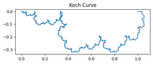
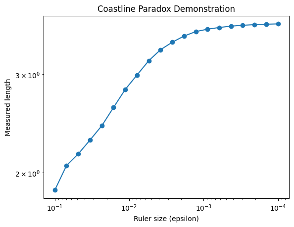
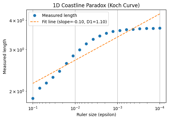
The figure above illustrates the coastline paradox using a Koch curve, a classic fractal curve. As the ruler size decreases, the measured length of the curve increases dramatically, highlighting that the “true” length of a jagged, self-similar shape is not well-defined. In the top plot, we visualise the Koch curve after six iterations, showing its intricate zig-zag pattern. The bottom plot demonstrates the paradox quantitatively: on a log–log scale, smaller ruler sizes (on the right) capture finer details, resulting in a rapidly increasing measured length. This simple experiment illustrates why fractal curves require a scale-invariant descriptor—the Minkowski or box-counting dimension—to characterise their complexity, rather than relying on a single length measurement.

The figures above illustrate the coastline paradox using a Koch curve, a classic fractal curve. As the ruler size decreases, the measured length of the curve increases dramatically, highlighting that the “true” length of a jagged, self-similar shape is not well-defined. In the top plot, we visualise the Koch curve after six iterations, showing its intricate zig-zag pattern. The bottom plot demonstrates the paradox quantitatively: on a log–log scale, smaller ruler sizes (on the right) capture finer details, resulting in a rapidly increasing measured length. This simple experiment illustrates why fractal curves require a scale-invariant descriptor—the Minkowski or box-counting dimension—to characterise their complexity, rather than relying on a single length measurement.

Mathematical Proof

Consider a jagged curve (e.g., a coastline) in 2D, and let $L(\varepsilon)$ denote the measured length using a ruler of size $\varepsilon$.

Divide the curve into segments of length $\varepsilon$. Let $N(\varepsilon)$ be the number of segments required to cover the curve:

$$L(\varepsilon) \approx N(\varepsilon) \cdot \varepsilon$$

Assume the curve is fractal with Minkowski–Bouligand dimension $D$, so the number of boxes needed to cover the curve scales as:

$$N(\varepsilon) \sim \varepsilon^{-D}$$

Substitute the scaling relation into the length formula:

$$L(\varepsilon) \sim \varepsilon \cdot \varepsilon^{-D} = \varepsilon^{1-D}$$

Interpretation:

If the curve is smooth: $D = 1$, then $L(\varepsilon) \sim \varepsilon^{0} = \text{constant}$.
If the curve is fractal: $D > 1$, then $L(\varepsilon) \to \infty$ as $\varepsilon \to 0$.

This demonstrates the paradox: the measured length depends on the ruler size, and only the fractal dimension $D$ provides a scale-invariant measure of the curve’s complexity.

Recovering the fractal dimension from data:

$$D = 1 - \frac{d \log L(\varepsilon)}{d \log \varepsilon}$$

On a log–log plot of $L(\varepsilon)$ vs $\varepsilon$, the slope is $1-D$.
This allows us to characterise the roughness of the curve quantitatively.

3D Coastline Paradox

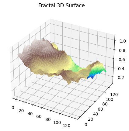
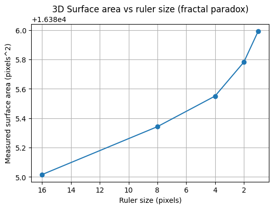
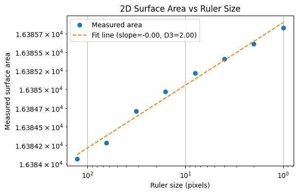
The figure below demonstrates the geographical area paradox, the 3D analogue of the coastline paradox. Here, we measure the surface area of a fractal terrain generated using the diamond-square algorithm. As the size of the measurement “ruler” (square grid) decreases, the measured surface area increases, revealing more of the fine-scale roughness of the terrain. Just as the length of a fractal curve diverges with smaller ruler sizes, the area of a fractal surface grows without bound. This shows that for rough surfaces, the conventional notion of area is ill-defined at very small scales. Instead, the fractal dimension of the surface provides a single, scale-invariant number that quantifies the complexity of the terrain.

Mathematical Formulation of the 3D Surface Paradox

Consider a 3D surface $z = f(x,y)$ defined over a 2D domain. Let $A(\varepsilon)$ denote the measured surface area using a square ruler of side $\varepsilon$.

Divide the plane into a grid of squares of side (\varepsilon). Let $N(\varepsilon)$ be the number of squares required to cover the surface (or, equivalently, the number of boxes intersecting the surface in 3D):

$$A(\varepsilon) \approx N(\varepsilon) \cdot \varepsilon^2$$

Assume the surface is fractal with Minkowski–Bouligand dimension $D$ (with $2 < D < 3$):

$$N(\varepsilon) \sim \varepsilon^{-D}$$

Substitute into the area formula:

$$A(\varepsilon) \sim \varepsilon^2 \cdot \varepsilon^{-D} = \varepsilon^{2-D}$$

Interpretation:

If the surface is smooth: $D = 2$, then $A(\varepsilon) \sim \varepsilon^0 = \text{constant}$.
If the surface is fractal: $D > 2$, then $A(\varepsilon) \to \infty$ as $\varepsilon \to 0$.

Recovering the fractal dimension from data:

$$D = 2 - \frac{d \log A(\varepsilon)}{d \log \varepsilon}$$

On a log–log plot of $A(\varepsilon)$ vs $\varepsilon$, the slope is $2$D.
This provides a scale-invariant measure of the surface’s roughness analogous to the 2D case but in two dimensions.

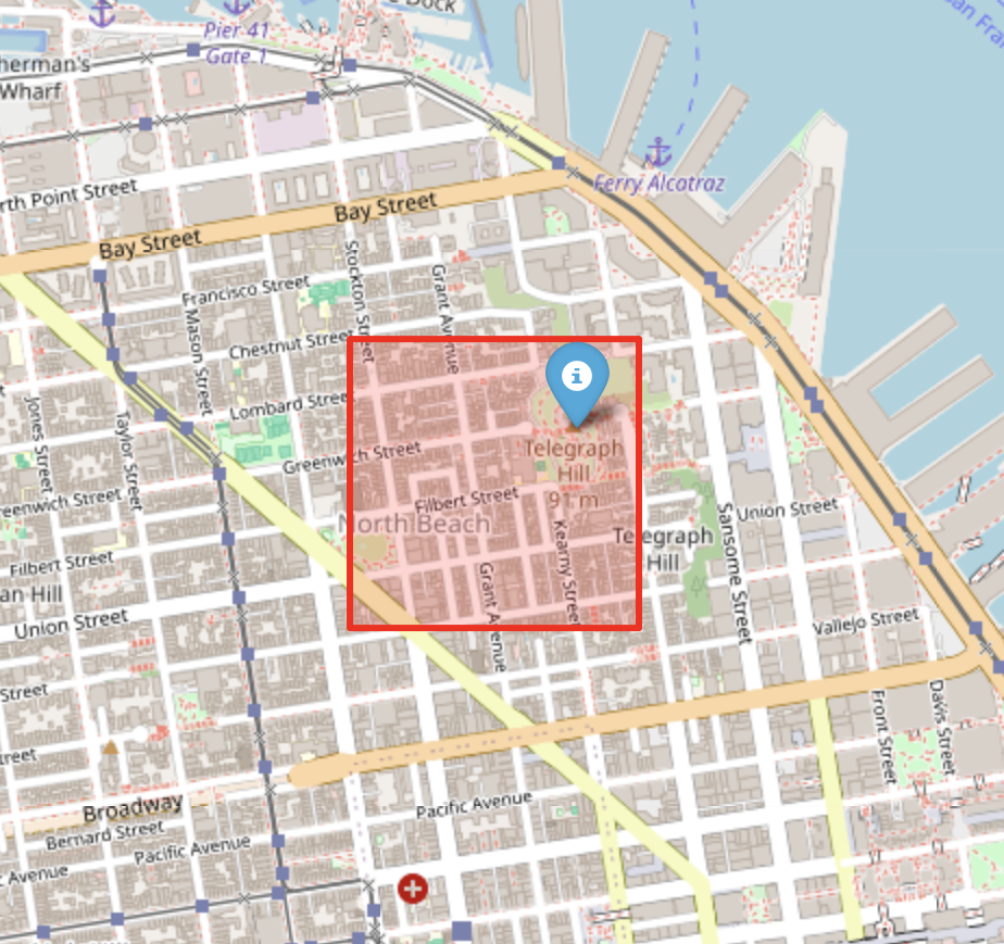
Telegraph Hill

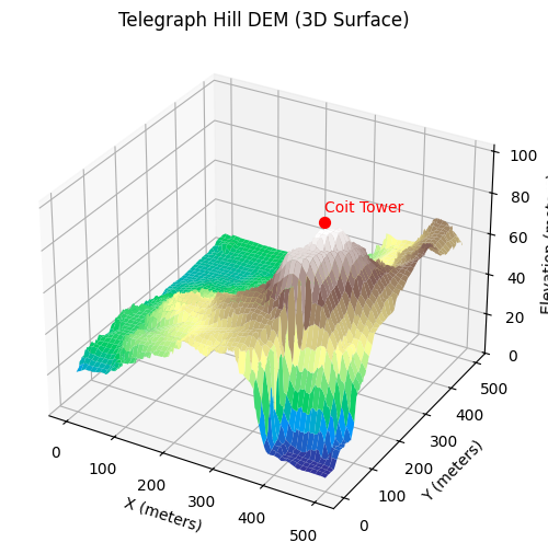
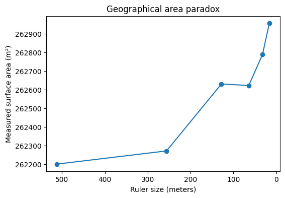
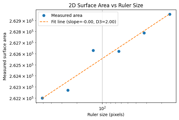
Up to this point, we have illustrated the coastline (or geographical area) paradox using a simulated fractal surface. While this is useful for building intuition, it is ultimately a controlled toy example. In this section, we replace the synthetic terrain with real elevation data from Telegraph Hill in San Francisco. Extracting and preparing this data turned out to be an ordeal in its own right—one that probably deserves a dedicated blog post. There is something uniquely satisfying about working with GIS data: every raster, projection, and coordinate transform is a walking demonstration of linear algebra in the wild. But I digress. With the elevation data in hand, we can now repeat the same multi-scale measurement exercise and observe the coastline paradox emerge not from a mathematical construction, but from an actual piece of geography.

To illustrate the coastline paradox in a real geographical setting, we estimate the surface area of Telegraph Hill using progressively smaller “rulers.” In the code above, the terrain is measured with square rulers of 256, 128, 64, and 32 meters, and the total surface area is recomputed at each scale. As the ruler size decreases, the measured area systematically increases. This is not because the hill is physically changing, but because finer rulers capture more of the terrain’s small-scale roughness—minor ridges, gullies, and local slope variations that are invisible at coarser resolutions. The resulting curve demonstrates the geographical area paradox: for a rough, fractal-like surface, area is not a single well-defined number, but a scale-dependent quantity. What remains invariant across scales is not the measured area itself, but the rate at which it grows as the ruler size shrinks—an idea formalised by the surface’s fractal dimension.

Fractional Dimensions

So far, we have seen how measured length or surface area depends on the ruler size: smaller rulers reveal more detail, producing larger measured values. The key insight of fractal geometry is that this scale-dependence can be quantified by a fractional, scale-invariant dimension, also called the Minkowski–Bouligand dimension.

2D Case: Koch Curve

For a fractal curve, the measured length (L(\varepsilon)) scales with ruler size (\varepsilon) as:

$$L(\varepsilon) \sim \varepsilon^{1-D_1} = 1.1$$

where $D_1$ is the fractal dimension of the curve. By plotting $\log L(\varepsilon)$ versus $\log \varepsilon$, the slope of the line gives $1-D_1$, from which we can solve for $D_1$. For the Koch curve, this yields $D_1 \approx 1.1$ (theoretically this is $1.26$), reflecting that the curve is “rougher than a line” but does not fill a plane.

3D Case: Simulated Fractal Surface

For a fractal surface, the measured area $A(\varepsilon)$ scales with ruler size $\varepsilon$ as:

$$A(\varepsilon) \sim \varepsilon^{2-D_2} = 2.00002$$

where (D_2) is the surface’s fractal dimension (with $2 < D_2 < 3$). A log–log plot of $A(\varepsilon)$ versus $\varepsilon$ gives a slope of $2-D_2$, allowing us to solve for $D_2$. In practice, simulated terrains often have $D_2 \approx 2.3{-}2.5$, meaning the surface is rougher than a plane but still does not fill 3D space.

Real-World Case: Telegraph Hill

Finally, we can apply the same method to elevation data from Telegraph Hill. Using square rulers of decreasing size, we measure the terrain’s surface area at each scale. A log–log plot of measured area versus ruler size produces a slope that corresponds to $2-D_{TH}$.

$$D_{TH} = 2 - \frac{d \log A(\varepsilon)}{d \log \varepsilon} = 2.00084$$

The resulting fractional dimension (D_{TH}) captures the true roughness of the hill, providing a quantitative, scale-invariant measure of the terrain’s complexity. Just like with the Koch curve or the simulated fractal surface, the hill exhibits a dimension that is between its topological dimension (2) and the embedding dimension (3), revealing the fractal nature of real-world landscapes.

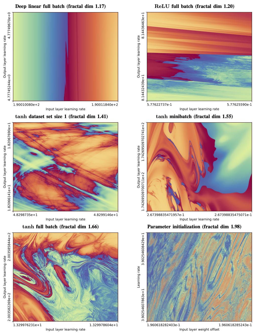
The Fractal Boundary of Trainability

The most interesting region of hyperparameter space is not where training clearly succeeds or clearly fails, but the boundary between the two. This is where learning rates are just stable enough, regularisation is just sufficient, and optimisation teeters on the edge of divergence.

When we zoom into this boundary between convergent (blue) and divergent (red) training regimes, something remarkable happens: structure appears at every scale. Regions that look smooth at coarse resolution reveal increasingly intricate patterns as we zoom in. No matter how closely we examine it, the boundary never simplifies.

In this sense, the boundary of neural network trainability behaves like a fractal. Just as with coastlines or rough surfaces, the distinction between “trainable” and “untrainable” depends on the scale at which we probe it — a reminder that even optimisation lives in a world of fractional geometry.

Scale dependent kinematics: spacetime extension

One intriguing extension is to imagine motion along a fractal path, where the effective distance depends on scale. If $L(\varepsilon) \sim \varepsilon^{1-D}$ is the measured length at scale $\varepsilon$, then a “scale-dependent velocity” $v(\varepsilon)$ could be written as:

$$v(\varepsilon) = \frac{dL(\varepsilon)}{dt} \sim \frac{\varepsilon^{1-D}}{dt}$$

For a particle moving in a fractal spacetime geometry, this hints at scale-dependent kinematics, where the observed velocity changes with the measurement resolution, connecting fractal dimension $D$ with the local structure of spacetime.

Conclusions and Final Thoughts

Through this exploration, we have seen how the coastline paradox extends naturally from 2D curves to 3D surfaces, and how it manifests in real-world terrain like Telegraph Hill. Starting with the Koch curve, we visualized the fundamental idea that measured length depends on the scale of measurement. Extending this to 3D, we saw that the surface area of a rough, fractal-like terrain increases as the measurement resolution becomes finer—a phenomenon we’ve called the geographical area paradox.

Applying the same principles to actual GIS data confirmed that this is not just a theoretical curiosity: hilly cities truly do have “more surface” at finer scales, and the apparent area depends on how finely it is measured.

Finally, this journey highlighted the importance of fractional dimensions. Traditional notions of dimension—1D, 2D, 3D—are insufficient to capture the complexity of fractal structures. By calculating Minkowski–Bouligand dimensions from 1D curves, 2D surfaces, and real-world elevation data, we gained a quantitative, scale-invariant measure of roughness.

In the end, the coastline paradox is more than a curiosity: it offers a window into the hidden complexity of the world, from jagged coastlines to hilly terrain, and pushes us to rethink the conventional notion of integer dimensions. Indeed, questioning our intuition about dimensions may be essential for a deeper understanding of concepts like velocity, especially when the underlying physical paths we traverse may be inherently fractal.

References

Locality, Learning, and the FFT: Why CNNs Avoid the Fourier Domain

2025-12-06T00:00:00.000Z

Introduction

Convolution sits at the heart of modern machine learning—especially convolutional neural networks (CNNs)—yet the underlying mathematics is often hidden behind highly optimised implementations in PyTorch, TensorFlow, and other frameworks. As a result, many of the properties that make convolution such a powerful building block for deep learning become obscured, particularly when we try to reason about model behaviour or debug a failing architecture.

If you know the convolution theorem, a natural question arises:

Why don’t CNNs simply compute a Fourier transform of the input and kernel, multiply them in the frequency domain, and invert the result? Wouldn’t that be simpler and faster?

This blog post addresses exactly that question. We will see that:

FFT-based convolution is not local.
In the Fourier domain every coefficient depends on every input pixel. This destroys the locality structure that CNNs rely on to learn hierarchical, spatially meaningful features. As a result, it breaks the very inductive bias that makes CNNs effective.
FFT-based convolution is not computationally cheaper in neural networks.
Although FFTs are asymptotically efficient, they must be recomputed on every forward and backward pass—and the cost of repeatedly transforming inputs, kernels, and gradients outweighs any benefit from spectral multiplication.

By the end of this post, we’ll have a clear, explicit comparison—both in matrix form and via backpropagation—showing why CNNs deliberately perform convolution in the spatial domain. Any practioner of signal processing should also be interested in knowing when the “locality” property is useful and when it is not!

1-D Convolution

Let us start with the most basic form of convolution, the 1D convolution. In this case you have a filter (which is nothing but a sequence of numbers) that you want to multiply with your signal in order to produce another signal which is hopefully more interesting to you. For example, in your headphones, you want to multiply a set of numbers with the music signal such that the resulting signal is more music than the wailing baby 1 row behind you.

import numpy as np

def conv1d_direct(x, h):
    nx, nh = len(x), len(h)
    y = np.zeros(nx+nh-1)
    for n in range(len(y)):
        for m in range(nx):
            k = n - m
            if 0 <= k < nh:
                y[n] += x[m] * h[k]
    return y

x = np.array([1.,2.,0.,-1.]) # this is the signal of music + baby wailing
h = np.array([0.5,1.,0.5]) # this is a filter that when multiplied with x makes it more music
conv1d_direct(x,h)

Convolution Theorem

This brings us to the convolution theorem wherein we can prove that the process of convolution i.e. multiplying window-wise h and x is mathematically equivalent to a simple multiplication between the fft of h and the fft of x.

def conv_via_fft(x,h):
    N = len(x)+len(h)-1
    X = np.fft.rfft(x,n=N)
    H = np.fft.rfft(h,n=N)
    return np.fft.irfft(X*H,n=N)

np.max(np.abs(conv1d_direct(x,h) - conv_via_fft(x,h)))
print(conv1d_direct(x,h))
print(conv_via_fft(x,h))

2-D Convolution

Just like before before we will convolve a 2D filter with a 2D signal in the spatial domain. We will then, try to do it using the FFT. We will verify that the convolution theorem does indeed work in the 2D space as well.

def conv2d_direct(img, ker):
    ih, iw = img.shape
    kh, kw = ker.shape
    out = np.zeros((ih+kh-1, iw+kw-1))
    for i in range(out.shape[0]):
        for j in range(out.shape[1]):
            for m in range(ih):
                for n in range(iw):
                    km, kn = i-m, j-n
                    if 0 <= km < kh and 0 <= kn < kw:
                        out[i,j] += img[m,n] * ker[km,kn]
    return out

img = np.array([[0,0,0,0],[0,1,2,0],[0,3,4,0],[0,0,0,0]])
ker = np.array([[1,2,1],[2,4,2],[1,2,1]])/16
conv2d_direct(img,ker)

Convolution Theorem 2D

In a similar way to the 1D case instead of windowing and multiplying, we can take the fft of the signal and the kernel and simply multiply.

def conv2d_fft(img,ker):
    H,W = img.shape
    Kh,Kw = ker.shape
    OH,OW = H+Kh-1, W+Kw-1
    IMG = np.fft.rfft2(img, s=(OH,OW))
    KER = np.fft.rfft2(ker, s=(OH,OW))
    return np.fft.irfft2(IMG*KER, s=(OH,OW))

out_d = conv2d_direct(img,ker)
out_f = conv2d_fft(img,ker)
np.max(np.abs(out_d - out_f))

So why do NNs not use the FFT?

In a neural network, convolution is used to generate feature maps that feed into the next layer. At first glance, the convolution theorem suggests a tempting shortcut: instead of sliding a kernel spatially, we could transform both the image and kernel into the frequency domain, multiply them element-wise, and transform the result back. The output would be mathematically equivalent—so why not do this inside CNNs?

It turns out there are two fundamental reasons:

Neural networks care about more than just the output—they care about how the output is produced.
During backpropagation, each filter weight is updated using gradients derived from local spatial features. This locality enables CNNs to learn hierarchies of edges, textures, shapes, and patterns.
In the Fourier domain, however, gradients flow through global Fourier coefficients. Every frequency component depends on every pixel, so the update for a single weight depends on the entire image. This destroys the spatial locality that CNNs rely on and eliminates the inductive bias that makes them effective.
The FFT is not “simpler” computationally for neural networks.
While FFTs are efficient in isolation, a CNN would need to repeatedly compute forward FFTs, spectral multiplications, and inverse FFTs—not just for the forward pass, but also for backpropagation.
When you count actual multiplications and transforms, the FFT approach is often more expensive, especially for small kernels (e.g., 3×3, 5×5), which dominate modern architectures.

In short: CNNs avoid the Fourier domain because it removes locality and adds computational overhead—both of which undermine the very reasons convolution works so well in deep learning.

2D Spatial Convolution as a Matrix Multiply

For our next trick we will show the exact way in which your hardware actually computes convolutions. Spoiler: it will be some kind of matrix multiplication. This is quite different from the way convolution is taught in the classroom where you usually convolve with a patch of pixels in the spatial domain and roll the kernel onto the next patch nearby. In reality, this whole process is just represented as one huge matrix multiply. It is very important to think about convolution in this way, as it makes approaching complex questions easier. Since looping over pixels is not a coherent mathematical approach whose complexity is easy to compute. Once it is expressed as a matrix multiply between to matrices we can directly use a formula to compute complexity. More importantly, GPUs work fast precisely because they can parallelize this matrix multiply (as opposed to parallizing various kinds of for-loop structures).

In this section, $X$ denotes the input image. It’s worth noting that most deep-learning libraries treat the 2D and 1D cases in essentially the same way: the very first step is to reshape the image into a long vector, commonly written as $\mathrm{vec}(X)$. This operation—often implemented as im2col in the source code—unrolls local patches of the image so that convolution can be expressed as a matrix–vector multiplication.

$$X =\begin{bmatrix}x_{11} & x_{12} & x_{13} & x_{14} \\x_{21} & x_{22} & x_{23} & x_{24} \\x_{31} & x_{32} & x_{33} & x_{34} \\x_{41} & x_{42} & x_{43} & x_{44}\end{bmatrix},\quad\mathrm{vec}(X) =\begin{bmatrix}x_{11} \\ x_{12} \\ x_{13} \\ x_{14} \\x_{21} \\ x_{22} \\ x_{23} \\ x_{24} \\x_{31} \\ x_{32} \\ x_{33} \\ x_{34} \\x_{41} \\ x_{42} \\ x_{43} \\ x_{44}\end{bmatrix}.$$

Let the $3\times 3$ kernel we are interested in convolving be:

$$W =\begin{bmatrix}w_{11} & w_{12} & w_{13} \\w_{21} & w_{22} & w_{23} \\w_{31} & w_{32} & w_{33}\end{bmatrix}.$$

The valid convolution output (size $2\times 2$) is (again im2col outputs a long vector that can be then transformed to an image on the other end):

$$\mathrm{vec}(Y)=\begin{bmatrix}y_{11} \\ y_{12} \\ y_{21} \\ y_{22} \\\end{bmatrix}.$$

We can express the convolution as a matrix multiply:

$$\mathrm{vec}(Y) = T(W)\ \mathrm{vec}(X),$$

where $T(W)$ is the Block-Toeplitz with Toeplitz Blocks (BTTB) matrix.

$$T(W) =\begin{bmatrix}\color{blue}{w_{11}} & \color{blue}{w_{12}} & \color{blue}{w_{13}} & 0& \color{blue}{w_{21}} & \color{blue}{w_{22}} & \color{blue}{w_{23}} & 0& \color{blue}{w_{31}} & \color{blue}{w_{32}} & \color{blue}{w_{33}} & 0& 0 & 0 & 0 & 0 \\[2mm]%0 & \color{blue}{w_{11}} & \color{blue}{w_{12}} & \color{blue}{w_{13}}& 0 & \color{blue}{w_{21}} & \color{blue}{w_{22}} & \color{blue}{w_{23}}& 0 & \color{blue}{w_{31}} & \color{blue}{w_{32}} & \color{blue}{w_{33}}& 0 & 0 & 0 & 0 \\[2mm]%0 & 0 & 0 & 0 & \color{blue}{w_{11}} & \color{blue}{w_{12}} & \color{blue}{w_{13}} & 0& \color{blue}{w_{21}} & \color{blue}{w_{22}} & \color{blue}{w_{23}} & 0& \color{blue}{w_{31}} & \color{blue}{w_{32}} & \color{blue}{w_{33}} & 0 \\[2mm]%0 & 0 & 0 & 0 & 0 & \color{blue}{w_{11}} & \color{blue}{w_{12}} & \color{blue}{w_{13}}& 0 & \color{blue}{w_{21}} & \color{blue}{w_{22}} & \color{blue}{w_{23}}& 0 & \color{blue}{w_{31}} & \color{blue}{w_{32}} & \color{blue}{w_{33}}\end{bmatrix}.$$

Expanded, the output entries are:

$$y_{11} =w_{11} x_{11} + w_{12} x_{12} + w_{13} x_{13} + w_{21} x_{21} + w_{22} x_{22} + w_{23} x_{23} + w_{31} x_{31} + w_{32} x_{32} + w_{33}x_{33}$$$$y_{12} =w_{11} x_{12} + w_{12} x_{13} + w_{13} x_{14} + w_{21} x_{22} + w_{22} x_{23} + w_{23} x_{24} + w_{31} x_{32} + w_{32} x_{33} + w_{33}x_{34}$$$$y_{21} =w_{11} x_{21} + w_{12} x_{22} + w_{13} x_{23} + w_{21} x_{31} + w_{22} x_{32} + w_{23} x_{33} + w_{31} x_{41} + w_{32} x_{42} + w_{33} x_{43}$$$$y_{22} =w_{11} x_{22} + w_{12} x_{23} + w_{13} x_{24} + w_{21} x_{32} + w_{22} x_{33} + w_{23} x_{34} + w_{31} x_{42} + w_{32} x_{43} + w_{33} x_{44}$$

Loss Backpropagation in Convolution

1D Convolution Example

Let the 1D convolution be:

$$y = T(w) x$$

where:

($x \in \mathbb{R}^6$) is the input
($w \in \mathbb{R}^3$) is the kernel
($y \in \mathbb{R}^4$) is the output (valid convolution)

Assume a scalar loss ($L(y)$).

Step 1: Gradient w.r.t Output

$$\frac{\partial L}{\partial y} =\begin{bmatrix}\frac{\partial L}{\partial y_1} \\\frac{\partial L}{\partial y_2} \\\frac{\partial L}{\partial y_3} \\\frac{\partial L}{\partial y_4}\end{bmatrix}.$$

Step 2: Gradient w.r.t Kernel

Construct the input Toeplitz matrix:

$$T_x =\begin{bmatrix}x_1 & x_2 & x_3 \\x_2 & x_3 & x_4 \\x_3 & x_4 & x_5 \\x_4 & x_5 & x_6\end{bmatrix}.$$

Then the gradient w.r.t the kernel is:

$$\frac{\partial L}{\partial w} = T_x^\top \frac{\partial L}{\partial y} =\begin{bmatrix}x_1 & x_2 & x_3 & x_4 \\x_2 & x_3 & x_4 & x_5 \\x_3 & x_4 & x_5 & x_6 \\\end{bmatrix}\begin{bmatrix}\frac{\partial L}{\partial y_1} \\\frac{\partial L}{\partial y_2} \\\frac{\partial L}{\partial y_3} \\\frac{\partial L}{\partial y_4}\end{bmatrix}.$$

Observation: Each kernel weight sees only the local patches of the input it touches, preserving locality.

Step 3: Gradient w.r.t Input

$$\frac{\partial L}{\partial x} = T(w)^\top \frac{\partial L}{\partial y}.$$

Again, each input element only receives gradient from the outputs it contributed to.

2D Convolution Example

Only for completeness, it should be clear that 1D and 2D is handled the same way using im2col

For 2D BTTB convolution:

$$\mathrm{vec}(Y) = T(W) \mathrm{vec}(X),$$

with scalar loss ($L(Y)$):

Gradient w.r.t kernel:

$$\frac{\partial L}{\partial W} = T_X^\top \frac{\partial L}{\partial \mathrm{vec}(Y)}$$

Gradient w.r.t input:

$$\frac{\partial L}{\partial \mathrm{vec}(X)} = T(W)^\top \frac{\partial L}{\partial \mathrm{vec}(Y)}$$

Observation

Each kernel weight is influenced only by the input pixels in the patch it was applied to
Each input pixel receives gradients only from outputs it contributed to
This is why CNNs learn localized features efficiently.

2D Fourier Transform Convolution as Matrix Multiplies

Similar to the spatial convolution case we will represent the Fourier transform as a sequence of matrix multiplies. The recipe is as follows,

Fourier Transform of Kernel
Fourier Transform of 2D Image
Elementwise Multiply in the Frequency Domain
Inverse Fourier Transform

These matrices can get quite huge, but I thought we need to see them explicitly to make understanding them a bit easier.

We assume:

$$X =\begin{bmatrix}x_{11} & x_{12} & x_{13} & x_{14}\\x_{21} & x_{22} & x_{23} & x_{24}\\x_{31} & x_{32} & x_{33} & x_{34}\\x_{41} & x_{42} & x_{43} & x_{44}\\\end{bmatrix},\qquadW =\begin{bmatrix}w_{11} & w_{12} & w_{13}\\w_{21} & w_{22} & w_{23}\\w_{31} & w_{32} & w_{33}\\\end{bmatrix}$$

Flatten row-major:

$$\mathrm{vec}(X)=\begin{bmatrix}x_{11}\\x_{12}\\x_{13}\\x_{14}\\x_{21}\\x_{22}\\x_{23}\\x_{24}\\x_{31}\\x_{32}\\x_{33}\\x_{34}\\x_{41}\\x_{42}\\x_{43}\\x_{44}\\\end{bmatrix},\qquad\mathrm{vec}(W)=\begin{bmatrix}w_{11}\\w_{12}\\w_{13}\\w_{21}\\w_{22}\\w_{23}\\w_{31}\\w_{32}\\w_{33}\\\end{bmatrix}.$$

The 2D DFT matrix for a 4×4 image (flattened row-major) is:

$$F_{k,n} = e^{-2\pi i \cdot kn/16},\qquad k,n = 0,\dots,15.$$$$F=\begin{bmatrix}1 & 1 & 1 & 1 & 1 & 1 & 1 & 1 & 1 & 1 & 1 & 1 & 1 & 1 & 1 & 1 \\1 & c_{1} - is_{1} & c_{2} - is_{2} & c_{3} - is_{3} & c_{4} - is_{4} & c_{5} - is_{5} & c_{6} - is_{6} & c_{7} - is_{7} & -1 & c_{9} - is_{9} & c_{10} - is_{10} & c_{11} - is_{11} & c_{12} - is_{12} & c_{13} - is_{13} & c_{14} - is_{14} & c_{15} - is_{15} \\1 & c_{2} - is_{2} & c_{4} - is_{4} & c_{6} - is_{6} & -1 & c_{10} - is_{10} & c_{12} - is_{12} & c_{14} - is_{14} & 1 & c_{2} - is_{2} & c_{4} - is_{4} & c_{6} - is_{6} & -1 & c_{10} - is_{10} & c_{12} - is_{12} & c_{14} - is_{14} \\1 & c_{3} - is_{3} & c_{6} - is_{6} & c_{9} - is_{9} & c_{12} - is_{12} & c_{15} - is_{15} & c_{18} - is_{18} & c_{21} - is_{21} & -1 & c_{27} - is_{27} & c_{30} - is_{30} & c_{33} - is_{33} & c_{36} - is_{36} & c_{39} - is_{39} & c_{42} - is_{42} & c_{45} - is_{45} \\1 & c_{4} - is_{4} & -1 & c_{12} - is_{12} & 1 & c_{20} - is_{20} & -1 & c_{28} - is_{28} & 1 & c_{36} - is_{36} & -1 & c_{44} - is_{44} & 1 & c_{52} - is_{52} & -1 & c_{60} - is_{60} \\1 & c_{5} - is_{5} & c_{10} - is_{10} & c_{15} - is_{15} & c_{20} - is_{20} & c_{25} - is_{25} & c_{30} - is_{30} & c_{35} - is_{35} & -1 & c_{45} - is_{45} & c_{50} - is_{50} & c_{55} - is_{55} & c_{60} - is_{60} & c_{65} - is_{65} & c_{70} - is_{70} & c_{75} - is_{75} \\1 & c_{6} - is_{6} & c_{12} - is_{12} & c_{18} - is_{18} & -1 & c_{30} - is_{30} & c_{36} - is_{36} & c_{42} - is_{42} & 1 & c_{54} - is_{54} & c_{60} - is_{60} & c_{66} - is_{66} & -1 & c_{78} - is_{78} & c_{84} - is_{84} & c_{90} - is_{90} \\1 & c_{7} - is_{7} & c_{14} - is_{14} & c_{21} - is_{21} & c_{28} - is_{28} & c_{35} - is_{35} & c_{42} - is_{42} & c_{49} - is_{49} & -1 & c_{63} - is_{63} & c_{70} - is_{70} & c_{77} - is_{77} & c_{84} - is_{84} & c_{91} - is_{91} & c_{98} - is_{98} & c_{105} - is_{105} \\1 & -1 & 1 & -1 & 1 & -1 & 1 & -1 & 1 & -1 & 1 & -1 & 1 & -1 & 1 & -1 \\1 & c_{9} - is_{9} & c_{18} - is_{18} & c_{27} - is_{27} & c_{36} - is_{36} & c_{45} - is_{45} & c_{54} - is_{54} & c_{63} - is_{63} & -1 & c_{81} - is_{81} & c_{90} - is_{90} & c_{99} - is_{99} & c_{108} - is_{108} & c_{117} - is_{117} & c_{126} - is_{126} & c_{135} - is_{135} \\1 & c_{10} - is_{10} & c_{20} - is_{20} & c_{30} - is_{30} & 1 & c_{50} - is_{50} & c_{60} - is_{60} & c_{70} - is_{70} & 1 & c_{90} - is_{90} & c_{100} - is_{100} & c_{110} - is_{110} & 1 & c_{130} - is_{130} & c_{140} - is_{140} & c_{150} - is_{150} \\1 & c_{11} - is_{11} & c_{22} - is_{22} & c_{33} - is_{33} & c_{44} - is_{44} & c_{55} - is_{55} & c_{66} - is_{66} & c_{77} - is_{77} & -1 & c_{99} - is_{99} & c_{110} - is_{110} & c_{121} - is_{121} & c_{132} - is_{132} & c_{143} - is_{143} & c_{154} - is_{154} & c_{165} - is_{165} \\1 & c_{12} - is_{12} & -1 & c_{36} - is_{36} & 1 & c_{60} - is_{60} & -1 & c_{84} - is_{84} & 1 & c_{108} - is_{108} & -1 & c_{132} - is_{132} & 1 & c_{156} - is_{156} & -1 & c_{180} - is_{180} \\1 & c_{13} - is_{13} & c_{26} - is_{26} & c_{39} - is_{39} & c_{52} - is_{52} & c_{65} - is_{65} & c_{78} - is_{78} & c_{91} - is_{91} & -1 & c_{117} - is_{117} & c_{130} - is_{130} & c_{143} - is_{143} & c_{156} - is_{156} & c_{169} - is_{169} & c_{182} - is_{182} & c_{195} - is_{195} \\1 & c_{14} - is_{14} & c_{28} - is_{28} & c_{42} - is_{42} & -1 & c_{70} - is_{70} & c_{84} - is_{84} & c_{98} - is_{98} & 1 & c_{126} - is_{126} & c_{140} - is_{140} & c_{154} - is_{154} & -1 & c_{182} - is_{182} & c_{196} - is_{196} & c_{210} - is_{210} \\1 & c_{15} - is_{15} & c_{30} - is_{30} & c_{45} - is_{45} & c_{60} - is_{60} & c_{75} - is_{75} & c_{90} - is_{90} & c_{105} - is_{105} & -1 & c_{135} - is_{135} & c_{150} - is_{150} & c_{165} - is_{165} & c_{180} - is_{180} & c_{195} - is_{195} & c_{210} - is_{210} & c_{225} - is_{225}\\\end{bmatrix}$$

Where

$$c_n = \cos\left(\frac{2\pi n}{16}\right), \qquad s_n = \sin\left(\frac{2\pi n}{16}\right).$$

1. Fourier Transform of the Kernel**

$$\hat{W} = F \mathrm{vec}(W_{padded})$$

where $W_{padded}$ is the 3×3 kernel zero-padded to 4×4. Explicitly:

$$\mathrm{vec}(W_{padded}) =\begin{bmatrix}w_{11}\\w_{12}\\w_{13}\\0\\w_{21}\\w_{22}\\w_{23}\\0\\w_{31}\\w_{32}\\w_{33}\\0\\0\\0\\0\\0\\\end{bmatrix}.$$

Then:

$$\hat{W} = F \mathrm{vec}(W_{padded}).$$

Take the first row,

$$\hat{W}_1 = w_{11} + w_{12} + w_{13} + w_{21} + w_{22} + w_{23} + w_{31} + w_{32} + w_{33}$$

2. Fourier Transform of the Image

$$\hat{X} = F \mathrm{vec}(X)$$

Take the first row,

$$\hat{X}_1 = x_{11} + x_{12} + x_{13} + x_{14} + x_{21} + x_{22} + x_{23} + x_{24} + x_{31} + x_{32} + x_{33} + x_{34} + x_{41} + x_{42} + x_{43} + x_{44}$$

3. Multiply (Elementwise) in Frequency Space

Define the frequency-domain product:

$$\hat{Y} = \hat{W} \odot \hat{X}$$

Written explicitly:

$$\hat{Y}=\begin{bmatrix}\hat{W}_1 \hat{X}_1 \\\hat{W}_2 \hat{X}_2 \\\vdots \\\hat{W}_{16} \hat{X}_{16}\end{bmatrix}$$

4. Inverse Fourier Transform

To return to spatial domain:

$$\mathrm{vec}(Y) = F^{-1} \hat{Y} = \frac{1}{16} F \hat{Y}$$

Explicitly:

$$\mathrm{vec}(Y)= \frac{1}{16}F\begin{bmatrix}\hat{W}_1 \hat{X}_1 \\\hat{W}_2 \hat{X}_2 \\\hat{W}_3 \hat{X}_3 \\\vdots \\\hat{W}_{16} \hat{X}_{16}\end{bmatrix}.$$

Thus the first row of the output looks like (the subscript is 11 because it will eventually be recast to an image),

$$y_{11} = \frac{1}{16} \left(\hat{W}_1 \hat{X}_1 + \hat{W}_2 \hat{X}_2 + \hat{W}_3 \hat{X}_3 + \cdots + \hat{W}_{16} \hat{X}_{16}\right)$$

We will try to focus on that first term on the RHS, $\hat{W}_1$, $\hat{X}_1$,

$$\hat{W}_1\hat{X}_1 = (w_{11} + w_{12} + w_{13} + w_{21} + w_{22} + w_{23} + w_{31} + w_{32} + w_{33}) \times (x_{11} + x_{12} + x_{13} + x_{14} + x_{21} + x_{22} + x_{23} + x_{24} + x_{31} + x_{32} + x_{33} + x_{34} + x_{41} + x_{42} + x_{43} + x_{44})$$$$y_{11} = \frac{1}{16} (w_{11} + w_{12} + w_{13} +\dots + w_{33}) \times (x_{11} + x_{12} + x_{13} +\dots + x_{42} + x_{43} + \textcolor{red}{x_{44}})$$

Compare this to $y_{11}$ from the spatial case, notice that the term $\textcolor{red}{x_{44}}$ is missing in the below expression,

$$y_{11} = w_{11} x_{11} + w_{12} x_{12} + w_{13} x_{13} + w_{21}x_{21} + w_{22} x_{22} + w_{23} x_{23}+ w_{31} x_{31} + w_{32} x_{32} + w_{33} x_{33}$$

Eventually these two values will be numerically the same! We know this from the convolution theorem. In the next section we will see that the contributing values matter to the gradient back propagation and that is where the two approaches will differ.

Gradient Comparison

FFT Gradient

$$\frac{\partial y_{11}}{\partial w_{11}} = \frac{1}{16} \left( x_{11} + x_{12} + x_{13} + \dots + x_{44} \right)$$

Notice that every input pixel contributes to the gradient of $w_{11}$.

Similarly for other weights, EVERY pixel contributes to the gradient.

$$\frac{\partial y_{11}}{\partial w_{ij}} = \frac{1}{16} \left( x_{11} + x_{12} + \dots + x_{44} \right), \quad \forall w_{ij}$$

Gradient in the Spatial Convolution Case

Notice that each update depends only on the pixel patch that it touches!

$$\frac{\partial L}{\partial w_{ij}} = \frac{\partial L}{\partial y_{11}} \cdot \frac{\partial y_{11}}{\partial w_{ij}} = \frac{\partial L}{\partial y_{11}} \cdot \frac{1}{16} \sum_{m=1}^{4} \sum_{n=1}^{4} x_{mn}$$$$\frac{\partial y_{11}}{\partial w_{11}} = x_{11}, \quad\frac{\partial y_{11}}{\partial w_{12}} = x_{12}, \quad\frac{\partial y_{11}}{\partial w_{13}} = x_{13},$$$$\frac{\partial y_{11}}{\partial w_{21}} = x_{21}, \quad\frac{\partial y_{11}}{\partial w_{22}} = x_{22}, \quad\frac{\partial y_{11}}{\partial w_{23}} = x_{23},$$$$\frac{\partial y_{11}}{\partial w_{31}} = x_{31}, \quad\frac{\partial y_{11}}{\partial w_{32}} = x_{32}, \quad\frac{\partial y_{11}}{\partial w_{33}} = x_{33}.$$

Gradient update for scalar loss L

$$\frac{\partial L}{\partial w_{ij}} = \frac{\partial L}{\partial y_{11}} \cdot \frac{\partial y_{11}}{\partial w_{ij}}.$$

Computational Comparison

Spatial Convolution

Suppose:

Input image: $X$ of size $N \times N$
Kernel: $W$ of size $K \times K$
Output: $Y$ of size $(N-K+1) \times (N-K+1)$

Number of multiplications

Each output pixel requires $K^2$ multiplications:

$$\text{Total multiplications} = (N-K+1)^2 \cdot K^2 \approx N^2 K^2 \quad \text{for } N \gg K$$

Linear in number of pixels and kernel size.
Memory access is local, cache-friendly.

FFT-based Convolution

Forward pass:

Zero-pad kernel to size $N \times N$
Compute 2D FFT of input and kernel: $O(N^2 \log N)$ each
Elementwise multiplication in Fourier domain: $O(N^2)$
Inverse FFT: $O(N^2 \log N)$

Total computational cost

$$\text{FFT convolution} \approx 2 \cdot O(N^2 \log N) + O(N^2) \sim O(N^2 \log N)$$

For small kernels $K \ll N$ $K^2 \ll \log N$, so:

$$N^2 K^2 \ll N^2 \log N$$

Spatial convolution is cheaper for small kernels, which is why CNNs prefer it.
FFT becomes advantageous only for very large kernels or very large images.

TL;DR

Spatial convolution is efficient for small kernels and preserves locality which is crucial for CNNs to learn hierarchies.
FFT convolution has global interactions, destroys the local inductive bias, and is only computationally advantageous for very large kernels.

Conclusion

We have seen that spatial convolution is not only computationally more efficient but also better suited to capturing the hierarchical structure inherent in most images. For instance, a face detection algorithm may rely on local patterns such as the triangle formed by the eyes and the nose. A kernel that focuses specifically on this local arrangement is highly effective because it preserves locality.

Conversely, in domains like recommendation systems, where data may be represented as a sparse matrix of product–user interactions, capturing global patterns can be more important. Here, the “local” interactions often correspond to users with strong connections, whereas broader, global patterns reveal trends across the entire system. In such contexts, FFT-based approaches—or methods that leverage global connectivity, like graph convolutional networks—can be more appropriate.

This contrast explains why spatial CNNs excel in image-based tasks, while GCNs or FFT-based methods are more suitable for graphs representing global interactions, such as those between users and products.

References & Further Reading

Spatial Convoluttions visualized
“A Beginner’s Guide to Convolutions” (Colah’s Blog) – A visual, intuitive introduction to convolution and receptive fields.
https://colah.github.io/posts/2014-07-Understanding-Convolutions/
“The Fast Fourier Transform (FFT): Most Ingenious Algorithm Ever?” (3Blue1Brown video) – A beautiful geometric explanation of the FFT.
https://www.youtube.com/watch?v=h7apO7q16V0&utm_source=chatgpt.com
“Convolutional Neural Networks for Visual Recognition” (Stanford CS231n) – Gold-standard material on spatial convolution.
https://cs231n.github.io/convolutional-networks/

Visualization & Signal Processing

Khan Academy – Fourier Series & Fourier Transform – Visual and interactive explanations of frequency-domain thinking.
https://www.khanacademy.org/math/differential-equations/fourier-series
DSP Guide (Free Online Book) – Clear, practical engineering-focused intuition on convolution and transforms.
https://www.dspguide.com/

Implementing FFT-based Convolution

PyTorch FFT Tutorial – How PyTorch performs FFT-based convolution behind the scenes.
https://pytorch.org/docs/stable/fft.html
SciPy signal.fftconvolve – Practical tool frequently used for 2D FFT convolution.
https://docs.scipy.org/doc/scipy/reference/generated/scipy.signal.fftconvolve.html

Graph Neural Networks & Spectral Methods

“A Friendly Introduction to Graph Neural Networks” (Stanford) – Excellent intuition about GCNs and why they differ from CNNs.
https://web.stanford.edu/class/cs224w/
“Spectral Graph Convolution Explained” (Medium) – Gentle intro to graph Laplacians and filtering.
https://medium.com/towards-data-science/spectral-graph-convolution-explained-6dddb6c1c2b0

Practical Engineering Notes

“Why FFT Convolution is Faster” (StackOverflow discussion) – Short, practical engineering explanation.
https://stackoverflow.com/questions/12665249/why-is-fft-convolution-faster
“im2col and GEMM: How CNNs Are Really Implemented” (DeepLearning.ai forums) – Helps connect the maths to real-world kernels.
https://community.deeplearning.ai/t/how-im2col-really-works/27659

Hot & Cold Spectral GCNs: How Graph Fourier Transforms Connect Heat Flow and Cold-Start Recommendations

2025-11-22T00:00:00.000Z

Introduction

I have always been obsessed with the Fourier Transform, it is in my opinion the single greatest invention in the history of mathematics. Check out this Veritasium video on it! Part of what makes the Fourier Transform so ubiquitous is that any function can be broken down into its component frequencies. What is less well known is that the definition of "frequency" is purely mathematical and applies to a broader class of mathematical objects than just functions! In this post I will try to provide some intuition and visualizations that expand the Fourier Transform to graphs, called the Graph Fourier Transform. Hopefully once that is clear, we will apply the Graph Fourier Transform in a Spectral Graph Convolution Network to model heat propagation in a toroidal surface.

Repo:
https://github.com/FranciscoRMendes/graph_networks/tree/main

Colab Notebook:
https://github.com/FranciscoRMendes/graph_networks/blob/main/GCN.ipynb

Classical Fourier Transform As A Special Case Of The Graph Fourier Transform

While there are many ways to view the Fourier Transform, the most revealing perspective is to regard it as multiplication of a discrete signal by a special matrix. This viewpoint is useful for several reasons.

Once a signal is discretised, it becomes a vector, and any linear operation on it can be represented as multiplication by a matrix.
A transform is therefore a change of basis: multiplying a vector by a matrix produces a new representation of the same data.
However, only a very small number of matrices yield transformed coordinates that are interpretable. The Fourier matrix $F$ is special because its columns correspond to pure oscillations, which are the eigenvectors of every shift-invariant operator.
A useful transform must also be invertible. After performing operations in the transformed domain, one should be able to recover the original signal exactly. The Fourier matrix satisfies $F^\ast F = N I$, which gives a simple inverse and perfect reconstruction.

Every transform follows the same general recipe:

choose a matrix whose columns represent meaningful basis vectors,
multiply the signal by this matrix,
interpret the transformed coefficients,
use the inverse matrix to return to the original domain.

DFT via the Discrete Laplacian Matrix

We start by deriving the DFT in matrix form for a discrete signal. We will use this as a basis to then derive the Graph Fourier Transform.
Consider a 1-D signal sampled at $n$ evenly spaced points: $$x = (x_0, x_1, \dots, x_{n-1})^\top.$$

The continuous Laplacian operator $-\frac{d^2}{dx^2}$ is approximated on a uniform grid by the finite-difference stencil $$f''(i) \approx f(i+1) - 2 f(i) + f(i-1).$$

With periodic boundary conditions, the discrete Laplacian becomes the circulant matrix (keep this in mind when we go to the graph case, we shall see later that this is exactly the Laplacian of a cycle graph):

$$L =\begin{bmatrix} 2 & -1 & 0 & \cdots & 0 & -1 \\ -1 & 2 & -1 & \cdots & 0 & 0 \\ 0 & -1 & 2 & \cdots & 0 & 0 \\ \vdots & \vdots & \vdots & \ddots & \vdots & \vdots \\ 0 & 0 & 0 & \cdots & 2 & -1 \\ -1 & 0 & 0 & \cdots & -1 & 2\end{bmatrix}$$

This matrix discretises the second derivative, $-\frac{d^2}{dx^2}$ on a circle.

Eigenvectors of the Discrete Laplacian

The eigenvectors of $L$ are the complex exponentials $$u_k(j) = \frac{1}{\sqrt{n}} e^{-2\pi i k j / n}, \qquad k = 0, \dots, n-1.$$

These form the DFT basis. Their corresponding eigenvalues are $$\lambda_k = 4 \sin^2\!\left( \frac{\pi k}{n} \right).$$

Thus the discrete Laplacian admits the decomposition $$L = F^\ast \Lambda F,$$ where $F$ is the DFT matrix and $\Lambda = \operatorname{diag}(\lambda_k)$.

Fourier Transform in Matrix Form

Define the DFT matrix $$F_{k,j} = \frac{1}{\sqrt{n}} e^{- 2\pi i k j / n}.$$

The discrete Fourier transform of $x$ is the unitary matrix–vector product $$\hat{x} = F x$$ and the inverse transform is $$x = F^\ast \hat{x}$$.

Interpretation

The classical Fourier transform is therefore the spectral decomposition of the discrete Laplacian on a 1-D grid. Its eigenvectors (complex exponentials) play the role of “frequencies,” and its eigenvalues correspond to squared frequencies: $$L u_k = \lambda_k u_k.$$

So what the heck was the convolution?

Convolution is a local, weighted sum operation over neighbouring inputs. On a 1D signal you would need to use windows and slide them over the signal using the weighted sum operation over all signals in the window.

However, by moving to the spectral domain using the graph Fourier transform, convolution reduces to a simple multiplication: $$\hat{x} = F x,$$ where $F$ is the matrix of eigenvectors of the graph Laplacian and $x$ is the signal on the nodes.

This is crucial because it allows us to avoid explicitly defining a complicated convolution operator. Instead, we can learn filters in the spectral domain that act directly on the eigencomponents of the signal, greatly simplifying the operation while retaining expressive power.

On a graph, performing such a convolution directly is highly nontrivial because the neighbourhoods are irregular. But what if we could mathematically transform the graph to another domain where the operation is a simple multiplcation?

are identical">

Complex Interactions - In this structure one can easily add edges between users and between products. Note in the matrix factorization case, this is not possible since $R$ is only users x items. To include more complex interactions you pay the price with a larger and larger matrix.
Graph Structure - Perhaps the most visually striking feature of graph neural networks is that they can leverage graph structure itself (see Figure 4). Matrix factorization cannot do so easily
Higher order interactions can be captured more intuitively than in the case of matrix factorization

Before implementing a GCN, it’s important to understand its potential benefits. In my experience, matrix factorization often provides good results quickly, and moving to GCNs makes sense only if matrix factorization has already shown promise. Another key factor is the size and richness of interactions. If the graph representation is primarily bipartite, adding user edges may not significantly enhance the recommender system. In retail, edges sometimes represented families, but these structures were often too small to be useful—giving different recommendations to family members like $11$ and $1$ is acceptable since family ties alone don’t imply similar consumption patterns. However, identifying influencers, such as nodes with high degrees connected to isolated nodes, could guide targeted discounts for products they might promote.

I would be remiss, if I did not add that ALL of these issues with matrix factorization can be fixed by tweaking the factorization in some way. In fact, a recent paper Unifying Graph Convolutional Networks as Matrix Factorization by Liu et. al. does exactly this and shows that this approach is even better than a GCN. Which is why I think that the biggest advantage of the GCN is not that it is “better” in some sense, but rather the richness of the graphical structure lends itself naturally to the problem of recommending products, even if that graphical structure can then be shown to be equivalent to some rather more complex and less intuitive matrix structure. I recommend the following experiment flow :

A Simple GCN model

Let us continue on from our adjacency matrix $A$ and try to build a simple ML model of an embedding, we could hypothesize that an embedding is linearly dependent on the adjacency matrix.

$$H = f(AWX + I_nWX)$$

The second additive term bears a bit of explaining. Since the adjacency matrix has a $0$ diagonal, a value of $0$ get multiplied with the node’s own features $x\in X$. To avoid this we add the node’s own feature matrix $X$ using the diagonal matrix.

We need to make another important adjustment to $A$, we need to divide each term in the adjacency matrix by the degree of each node. $$\tilde{A} = A + I_n$$ $$A \equiv \tilde{D}^\frac{1}{2}\tilde{A}\tilde{D}^\frac{1}{2}$$ At the risk of abusing notation, we redefine $A$ as some normalized form of the adjacency matrix after edges connecting each node with itself have been added to the graph. I like this notation because it emphasizes the fact that you do not need to do this, if you suspect that normalizing your nodes by their degree of connectivity is not important then you do not need to do this step (though it costs you nothing to do so). In retail, the degree of a user node refers to the number of products they consume, while the degree of a product node reflects the number of customers it reaches. A product may have millions of consumers, but even the most avid user node typically consumes far fewer, perhaps only hundreds of products.

Here $X = [X_{u}, X_{i}$]. $$H = [U V]$$

Here we can split the equations by the subgraphs for which they apply to,

$$H_u = f(A_u W_u X_u)$$ $$H_v = f(A_v W_v X_v)$$

Note the equivalence the matrix case, in the matrix case we have to stack it ourselves because of the way we set up the matrix, but in the case of a GCN $H$ is already $m\times n$ and represents embeddings of both users and items.

The likelihood of an interaction is,

$$\hat y_{ij} = H_u^T H_v$$

The loss function is,

$$L = \sum_{(u, i) \in \mathcal{I}} \left( y_{ui} - \hat{y}_{ui} \right)^2$$

We can substitute the components of $H$ to get a tight expression for optimizing loss,

$$L = \sum_{(u, i) \in \mathcal{I}} \left( y_{ui} - f(A_u W_u X_u)^T f(A_v W_v X_v)\right)^2$$

This is the main “result” of this blog post that you can equally look at this one layer GCN as a matrix factorization problem of the user-item interaction matrix but with the more complex looking low rank matrices on the right. In this sense, you can always create a matrix factorization that equates to the loss function of a GCN.

You can update parameters using SGD or some other technique. I will not get into that too much in this post.

Understanding the GCN equation

Equations 1 and 2 are the most important equations in the GCN framework. $W$ is some $(m+n) \times d$ set of weights that learn how to embed or encode the information contained in $X$ into $H$. For this one layer model, we are only considering values from the nodes that are one edge away, since the value of $h_i$ is only dependent on all the $x_j$‘s that are directly connected to it and its own $x_i$. However, if you then apply this operation again, $H$ now has all the information contained in all the nodes connected to it in its own $h_i$ but also so does every other nodes $h_k$.

$$H^0 = f(AW^0X + I_nW^0X)$$$$H^1 = f(AW^1H^0 + I_nW^1H^0)$$

More succinctly, $$H^1 = f(AW^1 f(AW^0X + I_nW^0X)+ I_nW^1H^0)$$

Equivalence to Matrix Factorization for a one layer GCN

You could just as easily have started with two random matrices $U$ and $V$ and optimize them using your favorite optimization algorithm and end up with the likelihood for interaction function,

$$\hat y_{ij} = U^T V \equiv H_u^T H_v$$

So you get the same outcome for a one layer GCN as you would from matrix factorization. Note that, it has been proved that even multi-layer GCNs are equivalent to matrix factorization but the matrix being factorized is not that easy to interpret.

Key Takeaways

The differences between MF and GCN really begin to take form when we go into multi-layerd GCNs. In the case of the one layer GCN the embeddings of $H^0$ are only influenced by the nodes connected to it. Thus the features of a customer node will be only influenced by the products that they buy, similarly, the product node will be only influenced by the customers who by them. However, for deeper neural networks :

2 layer: every customer’s embedding is influenced by the embeddings of the products they consume and the embeddings of other customers of the products they consume. Similarly, every product is influenced by the customers who consume that product as well as by the products of the customers who consume that product.
3 layer: every customers embedding is influenced by the products they consume, other customers of the products they consume and products consumed by other customers of the products they consume. Similarly, every product is influenced by the consumers of that product, as well as products of consumers of that product as well as products consumed by consumers of that product.

You can see where this is going, in most practical applications, there are only so many levels you need to go to get a good result. In my experience $2$ is the bare minimum (because $1$ is unlikely to do better than an MF, in fact they are equivalent) and $3$ is about how deep you can feasibly go without exploding the number of training parameters.

That leads to another critical point when considering GCNs, you really pay a price (in blood, mind you) for every layer deep you go. Consider the one layer case, you really have $n\times d$ and $n\times d'$ parameters to learn, because you have to learn both the weight matrix $W$ and the matrix of embeddings $H$. But the MF case you directly learn $H$. So if you were only going to go one layer deep you might as well use matrix factorization.

Going the other way, if you are considering more than $3$ layers the reality of the problem (in my usual signal processing problems this would be “physical” laws) i.e. the behavioral constraints mean that more than 3 degrees deep of influence (think about what point 3 would mean for a $5$ layer network) is unlikely to be supported by any theoretical evidence of consumer behavior.

Final Prayer and Blessing

I would like for the reader of this to leave with a better sense of the relationship between matrix factorization and GCNs. Like most neural network based models we tend to think of them as a black box and a black box that is “better”. However, in the one layer GCN case we can see that they are equal, with the GCN in fact having more learnable parameters (therefore more cost to train).
Therefore, it makes sense to use $2$ layers or more. But when using more, we need to justify them either behaviorally or with expert advice.

How to go from MF to GCNs

Start with matrix factorization of the user-item matrix, maybe add in context or time. If it performs well and recommendations line up with non-ML recommendations (using base segmentation analysis), that means the model is at least somewhat sensible.
Consider doing a GCN next if the performance of MF is decent but not great. Additionally, definitely try GCN if you know (from marketing etc) that the richness of the graph structure actually plays a role in the prediction. For example, in the sale of Milwaukee tools a graph structure is probably not that useful. However, for selling Thursday Boots which is heavily influenced by social media clusters, the graph structure might be much more useful.
Interestingly, the MF matrices tend to be very long and narrow (there are usually thousands of users and most companies have far more users than they have products. This is not true for a company like Amazon (300 million users and 300 million products). But if you have a long narrow matrix that is sparse you are not too concerned with computation since at worst you have $m\times n \approx O(n), m<

It is worthwhile in a consulting environment to always start with a simple matrix factorization, the GCN for simplicity of use and understanding but then find a matrix structure that approximates only the most interesting and rich aspects of the graph structure that actually influence the final recommendations.

References

https://jonathan-hui.medium.com/graph-convolutional-networks-gcn-pooling-839184205692
https://tkipf.github.io/graph-convolutional-networks/ https://openreview.net/forum?id=HJxf53EtDr
https://distill.pub/2021/gnn-intro/ https://jonathan-hui.medium.com/graph-convolutional-networks-gcn-pooling-839184205692

Part III : What does Low Rank Factorization of a Convolutional Layer really do?

2024-09-13T00:00:00.000Z

Series

Low-Rank Approximation for Neural Networks

Part II : Shrinking Neural Networks for Embedded Systems Using Low Rank Approximations (LoRA)
Part III : What does Low Rank Factorization of a Convolutional Layer really do?
Part I : Shrinking Neural Networks for Embedded Systems Using Low Rank Approximations (LoRA)

Decomposition of a Convolutional layer

In Part I I described (in some detail) what it means to decompose a matrix multiply into a sequence of low rank matrix multiplies, and Part II extended that to convolutional kernels and rank selection. We can go further still for general tensors, though this is somewhat less easy to see since tensors in higher dimensions are quite hard to visualize.
Recall, the matrix formulation,

$$Y = XW + b = XUSV' + b$$

Where $U$ and $V$ are the left and right singular vectors of $W$ respectively. The idea is to approximate $W$ as a sum of outer products of $U$ and $V$ of lower rank.
Now instead of a weight matrix multiplication $y = WX + b$ we have a kernel operation, $y = K\circledast X + b$ where $\circledast$ is the convolution operation. The idea is to approximate $K$ as a sum of outer products of $U$ and $V$ of lower rank.
Interestingly, you can also think about this as a matrix multiplication, by creating a Toplitz matrix version of $K$ , call it $K'$ and then doing $y = K'X + b$. But this comes with issues as $K'$ is much much bigger than $K$. So we just approach it as a convolution operation for now.

Convolution Operation

At the heart of it, a convolution operation takes a smaller cube subset of a “cube” of numbers (also known as the map stack) multiplies each of those numbers by a fixed set of numbers (also known as the kernel) and gives a single scalar output. Let us start with what each “slice” of the cube really represents.

Now that we have a working example of the representation, let us try to visualize what a convolution is.

A convolution operation takes a subset of the RGB image across all channels and maps it to one number (a scalar), by multiplying the cube of numbers with a fixed set of numbers (a.k.a kernel, not pictured here) and adding them together.A convolution operation multiplies each pixel in the image across all $3$ channels with a fixed number and add it all up.

Low Rank Approximation of Convolution

Now that we have a good idea of what a convolution looks like, we can now try to visualize what a low rank approximation to a convolution might look like. The particular kind of approximation we have chosen here does the following 4 operations to approximate the one convolution operation being done.

Painful Example of Convolution by hand

Consider the input matrix :

$$X = \begin{bmatrix}1 & 2 & 3 & 0 & 1 \\0 & 1 & 2 & 3 & 0 \\3 & 0 & 1 & 2 & 3 \\2 & 3 & 0 & 1 & 2 \\1 & 2 & 3 & 0 & 1 \\\end{bmatrix}$$ Input slice: $$\begin{bmatrix}1 & 2 & 3 \\0 & 1 & 2 \\3 & 0 & 1 \\\end{bmatrix}$$

Kernel: $$\begin{bmatrix}1 & 0 & -1 \\1 & 0 & -1 \\1 & 0 & -1 \\\end{bmatrix}$$

Element-wise multiplication and sum: $$(1 \cdot 1) + (2 \cdot 0) + (3 \cdot -1) + \\(0 \cdot 1) + (1 \cdot 0) + (2 \cdot -1) + \\(3 \cdot 1) + (0 \cdot 0) + (1 \cdot -1)$$

$$\implies1 + 0 - 3 + \\0 + 0 - 2 + \\3 + 0 - 1 = -2$$ Now repeat that by moving the kernel one step over (you can in fact change this with the stride argument for convolution).

Low Rank Approximation of convolution

Now we will painfully do a low rank decomposition of the convolution kernel above. There is a theorem that says that a $2D$ matrix can be approximated by a sum of 2 outer products of two vectors. Say we can express $K$ as, $$K \approx a_1 \times b_1 + a_2\times b_2$$

We can easily guess $a_i, b_i$. Consider, $$a_1 = \begin{bmatrix} 1\\ 1\\ 1\\ \end{bmatrix}$$ $$b_1 = \begin{bmatrix} 1\\ 0\\ -1\\ \end{bmatrix}$$ $$a_2 = \begin{bmatrix} 0\\ 0\\ 0\\ \end{bmatrix}$$ $$b_2 = \begin{bmatrix} 0\\ 0\\ 0\\ \end{bmatrix}$$

This is easy because I chose values for the kernel that were easy to break down. How to perform this breakdown is the subject of the later sections.

$$K = a_1\times b_1 + a_2 \times b_2 = \begin{bmatrix}1 & 0& -1 \\1 & 0 & -1 \\1 & 0 & -1 \\\end{bmatrix} +\begin{bmatrix}0 & 0 & 0 \\0 & 0 & 0 \\0 & 0 & 0 \\\end{bmatrix} = \begin{bmatrix}1 & 0 & -1 \\1 & 0 & -1 \\1 & 0 & -1 \\\end{bmatrix}$$

Consider the original kernel matrix $K$ and the low-rank vectors:

$$K = \begin{bmatrix}1 & 0 & -1 \\1 & 0 & -1 \\1 & 0 & -1\end{bmatrix}$$$$a_1 = \begin{bmatrix}1 \\1 \\1\end{bmatrix}, \quadb_1 = \begin{bmatrix}1 \\0 \\-1\end{bmatrix}$$

The input matrix $M$ is:

$$M = \begin{bmatrix}1 & 2 & 3 & 0 & 1 \\0 & 1 & 2 & 3 & 0 \\3 & 0 & 1 & 2 & 3 \\2 & 3 & 0 & 1 & 2 \\1 & 2 & 3 & 0 & 1\end{bmatrix}$$

Convolution with Original Kernel

Perform the convolution at the top-left corner of the input matrix:

$$\text{Input slice} = \begin{bmatrix}1 & 2 & 3 \\0 & 1 & 2 \\3 & 0 & 1\end{bmatrix}$$$$\text{Element-wise multiplication and sum:}$$$$\begin{aligned}(1 \times 1) + (2 \times 0) + (3 \times -1) + \\(0 \times 1) + (1 \times 0) + (2 \times -1) + \\(3 \times 1) + (0 \times 0) + (1 \times -1) &= \\1 + 0 - 3 + 0 + 0 - 2 + 3 + 0 - 1 &= -2\end{aligned}$$

Convolution with Low-Rank Vectors

Using the low-rank vectors:

$$a_1 = \begin{bmatrix}1 \\1 \\1\end{bmatrix}, \quadb_1 = \begin{bmatrix}1 \\0 \\-1\end{bmatrix}$$

Step 1: Apply $b_1$ (filter along the columns):**

$$\text{Column-wise operation:}$$$$\begin{aligned}1 \cdot \begin{bmatrix}1 \\0 \\-1\end{bmatrix} &= \begin{bmatrix}1 \\0 \\-1\end{bmatrix} \\2 \cdot \begin{bmatrix}1 \\0 \\-1\end{bmatrix} &= \begin{bmatrix}2 \\0 \\-2\end{bmatrix} \\3 \cdot \begin{bmatrix}1 \\0 \\-1\end{bmatrix} &= \begin{bmatrix}3 \\0 \\-3\end{bmatrix}\end{aligned}$$$$\text{Summed result for each column:}$$$$\begin{bmatrix}1 \\0 \\-1\end{bmatrix} +\begin{bmatrix}2 \\0 \\-2\end{bmatrix} +\begin{bmatrix}3 \\0 \\-3\end{bmatrix} =\begin{bmatrix}6 \\0 \\-6\end{bmatrix}$$

Step 2: Apply $a_1$ (sum along the rows):**

$$\text{Row-wise operation:}$$$$1 \cdot (6) + 1 \cdot (0) + 1 \cdot (-6) = 6 + 0 - 6 = 0$$

Comparison

Convolution with Original Kernel: -2
Convolution with Low-Rank Vectors: 0

The results are different due to the simplifications made by the low-rank approximation. But this is part of the problem that we need to optimize for when picking low rank approximations. In practice, we will ALWAYS lose some accuracy

PyTorch Implementation

Below you can find the original definition of AlexNet.

class Net(nn.Module):
    def __init__(self):
        super().__init__()
        self.layers  = nn.ModuleDict()
        self.layers['conv1'] = nn.Conv2d(3, 6, 5)
        self.layers['pool'] = nn.MaxPool2d(2, 2)
        self.layers['conv2'] = nn.Conv2d(6, 16, 5)
        self.layers['fc1'] = nn.Linear(16 * 5 * 5, 120)
        self.layers['fc2'] = nn.Linear(120, 84)
        self.layers['fc3'] = nn.Linear(84, 10)

    def forward(self,x):
        x = self.layers['pool'](F.relu(self.layers['conv1'](x)))
        x = self.layers['pool'](F.relu(self.layers['conv2'](x)))
        x = torch.flatten(x, 1)
        x = F.relu(self.layers['fc1'](x))
        x = F.relu(self.layers['fc2'](x))
        x = self.layers['fc3'](x)
        return x

def evaluate_model(net):
    import torchvision.transforms as transforms
    batch_size = 4 # [4, 3, 32, 32]
    transform = transforms.Compose(
        [transforms.ToTensor(),
         transforms.Normalize((0.5, 0.5, 0.5), (0.5, 0.5, 0.5))])
    classes = ('plane', 'car', 'bird', 'cat',
               'deer', 'dog', 'frog', 'horse', 'ship', 'truck')
    trainset = torchvision.datasets.CIFAR10(root='../data', train=True,
                                            download=True, transform=transform)
    trainloader = torch.utils.data.DataLoader(trainset, batch_size=batch_size,
                                              shuffle=True, num_workers=2)
    testset = torchvision.datasets.CIFAR10(root='../data', train=False,
                                           download=True, transform=transform)
    testloader = torch.utils.data.DataLoader(testset, batch_size=batch_size,
                                             shuffle=False, num_workers=2)
    # prepare to count predictions for each class
    correct_pred = {classname: 0 for classname in classes}
    total_pred = {classname: 0 for classname in classes}
    # again no gradients needed
    with torch.no_grad():
        for data in testloader:
            images, labels = data
            outputs = net(images)
            _, predictions = torch.max(outputs, 1)
            # collect the correct predictions for each class
            for label, prediction in zip(labels, predictions):
                if label == prediction:
                    correct_pred[classes[label]] += 1
                total_pred[classes[label]] += 1
    # print accuracy for each class
    for classname, correct_count in correct_pred.items():
        accuracy = 100 * float(correct_count) / total_pred[classname]
        print(f'Original Accuracy for class: {classname:5s} is {accuracy:.1f} %')

Now let us decompose the first convolutional layer into 3 simpler layers using SVD


def slice_wise_svd(tensor,rank):
    # tensor is a 4D tensor
    # rank is the target rank
    # returns a list of 4D tensors
    # each tensor is a slice of the input tensor
    # each slice is decomposed using SVD
    # and the decomposition is used to approximate the slice
    # the approximated slice is returned as a 4D tensor
    # the list of approximated slices is returned
    num_filters, input_channels, kernel_width, kernel_height = tensor.shape
    kernel_U = torch.zeros((num_filters, input_channels,kernel_height,rank))
    kernel_S = torch.zeros((input_channels,num_filters,rank,rank))
    kernel_V = torch.zeros((num_filters,input_channels,rank,kernel_width))
    approximated_slices = []
    reconstructed_tensor = torch.zeros_like(tensor)
    for i in range(num_filters):
        for j in range(input_channels):
            U, S, V = torch.svd(tensor[i, j,:,:])
            U = U[:,:rank]
            S = S[:rank]
            V = V[:,:rank]
            kernel_U[i,j,:,:] = U
            kernel_S[j,i,:,:] = torch.diag(S)
            kernel_V[i,j,:,:] = torch.transpose(V,0,1)


    # print the reconstruction error
    print("Reconstruction error: ",torch.norm(reconstructed_tensor-tensor).item())

    return kernel_U, kernel_S, kernel_V

def svd_decomposition_conv_layer(layer, rank):
    """ Gets a conv layer and a target rank,
        returns a nn.Sequential object with the decomposition
    """

    # Perform SVD decomposition on the layer weight tensorly.
    
    layer_weight = layer.weight.data
    kernel_U, kernel_S, kernel_V = slice_wise_svd(layer_weight,rank)
    U_layer = nn.Conv2d(in_channels=kernel_U.shape[1],
                                                out_channels=kernel_U.shape[0], kernel_size=(kernel_U.shape[2], 1), padding=0, stride = 1,
                                                dilation=layer.dilation, bias=True)
    S_layer = nn.Conv2d(in_channels=kernel_S.shape[1],
                                                out_channels=kernel_S.shape[0], kernel_size=1, padding=0, stride = 1,
                                                dilation=layer.dilation, bias=False)
    V_layer = nn.Conv2d(in_channels=kernel_V.shape[1],
                                                out_channels=kernel_V.shape[0], kernel_size=(1, kernel_V.shape[3]), padding=0, stride = 1,
                                                dilation=layer.dilation, bias=False)
    # store the bias in U_layer from layer
    U_layer.bias = layer.bias

    # set weights as the svd decomposition
    U_layer.weight.data = kernel_U
    S_layer.weight.data = kernel_S
    V_layer.weight.data = kernel_V

    return [U_layer, S_layer, V_layer]
    
    
class lowRankNetSVD(Net):
    def __init__(self, original_network):
        super().__init__()
        self.layers = nn.ModuleDict()
        self.initialize_layers(original_network)
    
    def initialize_layers(self, original_network):
        # Make deep copy of the original network so that it doesn't get modified
        og_network = copy.deepcopy(original_network)
        # Getting first layer from the original network
        layer_to_replace = "conv1"
        # Remove the first layer
        for i, layer in enumerate(og_network.layers):
            if layer == layer_to_replace:
                # decompose that layer
                rank = 1
                kernel = og_network.layers[layer].weight.data
                decomp_layers = svd_decomposition_conv_layer(og_network.layers[layer], rank)
                for j, decomp_layer in enumerate(decomp_layers):
                    self.layers[layer + f"_{j}"] = decomp_layer
            else:
                self.layers[layer] = og_network.layers[layer]
    
    def forward(self, x):
        x = self.layers['conv1_0'](x)
        x = self.layers['conv1_1'](x)
        x = self.layers['conv1_2'](x)
        x = self.layers['pool'](F.relu(x))
        x = self.layers['pool'](F.relu(self.layers['conv2'](x)))
        x = torch.flatten(x, 1)
        x = F.relu(self.layers['fc1'](x))
        x = F.relu(self.layers['fc2'](x))
        x = self.layers['fc3'](x)
        return x

Decomposition into a list of simpler operations

The examples above are quite simple and are perfectly good for simplifying neural networks. This is still an active area of research. One of the things that researchers try to do is try to further simplify each already simplified operation, of course you pay the price of more operations. The one we will use for this example is one where the operations is broken down into four simpler operations.

(Green) Takes one pixel from the image across all $3$ channels and maps it to one value
(Red) Takes one long set of pixels from one channel and maps it to one value
(Blue) Takes one wide set of pixels from one channel and maps it to one value
(Green) takes one pixel from all $3$ channels and maps it to one value

Intuitively, we are still taking the subset “cube” but we have broken it down so that in any given operation only $1$ dimension is not $1$. This is really the key to reducing the complexity of the initial convolution operation, because even though there are more such operations each operations is more complex.

PyTorch Implementation

In this section, we will take AlexNet (Net), evaluate (evaluate_model) it on some data and then decompose the convolutional layers.

Declaring both the original and low rank network

Here we will decompose the second convolutional layer, given by the layer_to_replace argument. The two important lines to pay attention to are est_rank and cp_decomposition_conv_layer. The first function estimates the rank of the convolutional layer and the second function decomposes the convolutional layer into a list of simpler operations.

class lowRankNet(Net):

    def __init__(self, original_network):
        super().__init__()
        self.layers = nn.ModuleDict()
        self.initialize_layers(original_network)

    def initialize_layers(self, original_network):
        # Make deep copy of the original network so that it doesn't get modified
        og_network = copy.deepcopy(original_network)
        # Getting first layer from the original network
        layer_to_replace = "conv2"
        # Remove the first layer
        for i, layer in enumerate(og_network.layers):
            if layer == layer_to_replace:
                # decompose that layer
                rank = est_rank(og_network.layers[layer])
                decomp_layers = cp_decomposition_conv_layer(og_network.layers[layer], rank)
                for j, decomp_layer in enumerate(decomp_layers):
                    self.layers[layer + f"_{j}"] = decomp_layer
            else:
                self.layers[layer] = og_network.layers[layer]
        # Add the decomposed layers at the position of the deleted layer

    def forward(self, x, layer_to_replace="conv2"):
        x = self.layers['pool'](F.relu(self.layers['conv1'](x)))
        # x = self.layers['pool'](F.relu(self.laye['conv2'](x)
        x = self.layers['conv2_0'](x)
        x = self.layers['conv2_1'](x)
        x = self.layers['conv2_2'](x)
        x = self.layers['pool'](F.relu(self.layers['conv2_3'](x)))
        x = torch.flatten(x, 1)
        x = F.relu(self.layers['fc1'](x))
        x = F.relu(self.layers['fc2'](x))
        x = self.layers['fc3'](x)
        return x

Evaluate the Model

You can evaluate the model by running the following code. This will print the accuracy of the original model and the low rank model.

decomp_alexnet = lowRankNetSVD(net)
# replicate with original model

correct_pred = {classname: 0 for classname in classes}
total_pred = {classname: 0 for classname in classes}

# again no gradients needed
with torch.no_grad():
    for data in testloader:
        images, labels = data
        outputs = decomp_alexnet(images)
        _, predictions = torch.max(outputs, 1)
        # collect the correct predictions for each class
        for label, prediction in zip(labels, predictions):
            if label == prediction:
                correct_pred[classes[label]] += 1
            total_pred[classes[label]] += 1

# print accuracy for each class
for classname, correct_count in correct_pred.items():
    accuracy = 100 * float(correct_count) / total_pred[classname]
    print(f'Lite Accuracy for class: {classname:5s} is {accuracy:.1f} %')

Let us first discuss estimate rank. For a complete discussion see the the references by Nakajima and Shinchi. The basic idea is that we take the tensor, “unfold” it along one axis (basically reduce the tensor into a matrix by collapsing around other axes) and estimate the rank of that matrix.
You can find est_rank below.

from __future__ import division
import torch
import numpy as np
# from scipy.sparse.linalg import svds
from scipy.optimize import minimize_scalar
import tensorly as tl

def est_rank(layer):
    W = layer.weight.data
    # W = W.detach().numpy() #the weight has to be a numpy array for tl but needs to be a torch tensor for EVBMF
    mode3 = tl.base.unfold(W.detach().numpy(), 0)
    mode4 = tl.base.unfold(W.detach().numpy(), 1)
    diag_0 = EVBMF(torch.tensor(mode3))
    diag_1 = EVBMF(torch.tensor(mode4))

    # round to multiples of 16
    multiples_of = 8 # this is done mostly to standardize the rank to a standard set of numbers, so that 
    # you do not end up with ranks 7, 9 etc. those would both be approximated to 8.
    # that way you get a sense of the magnitude of ranks across multiple runs and neural networks
    # return int(np.ceil(max([diag_0.shape[0], diag_1.shape[0]]) / 16) * 16)
    return int(np.ceil(max([diag_0.shape[0], diag_1.shape[0]]) / multiples_of) * multiples_of)

def EVBMF(Y, sigma2=None, H=None):
    """Implementation of the analytical solution to Empirical Variational Bayes Matrix Factorization.
    This function can be used to calculate the analytical solution to empirical VBMF.
    This is based on the paper and MatLab code by Nakajima et al.:
    "Global analytic solution of fully-observed variational Bayesian matrix factorization."

    Notes
    -----
        If sigma2 is unspecified, it is estimated by minimizing the free energy.
        If H is unspecified, it is set to the smallest of the sides of the input Y.

    Attributes
    ----------
    Y : numpy-array
        Input matrix that is to be factorized. Y has shape (L,M), where L<=M.

    sigma2 : int or None (default=None)
        Variance of the noise on Y.

    H : int or None (default = None)
        Maximum rank of the factorized matrices.

    Returns
    -------
    U : numpy-array
        Left-singular vectors.

    S : numpy-array
        Diagonal matrix of singular values.

    V : numpy-array
        Right-singular vectors.

    post : dictionary
        Dictionary containing the computed posterior values.


    References
    ----------
    .. [1] Nakajima, Shinichi, et al. "Global analytic solution of fully-observed variational Bayesian matrix factorization." Journal of Machine Learning Research 14.Jan (2013): 1-37.

    .. [2] Nakajima, Shinichi, et al. "Perfect dimensionality recovery by variational Bayesian PCA." Advances in Neural Information Processing Systems. 2012.
    """
    L, M = Y.shape  # has to be L<=M

    if H is None:
        H = L

    alpha = L / M
    tauubar = 2.5129 * np.sqrt(alpha)

    # SVD of the input matrix, max rank of H
    U, s, V = torch.svd(Y)
    U = U[:, :H]
    s = s[:H]
    V[:H].t_()

    # Calculate residual
    residual = 0.
    if H < L:
        residual = torch.sum(torch.sum(Y ** 2) - torch.sum(s ** 2))

    # Estimation of the variance when sigma2 is unspecified
    if sigma2 is None:
        xubar = (1 + tauubar) * (1 + alpha / tauubar)
        eH_ub = int(np.min([np.ceil(L / (1 + alpha)) - 1, H])) - 1
        upper_bound = (torch.sum(s ** 2) + residual) / (L * M)
        lower_bound = np.max([s[eH_ub + 1] ** 2 / (M * xubar), torch.mean(s[eH_ub + 1:] ** 2) / M])

        scale = 1.  # /lower_bound
        s = s * np.sqrt(scale)
        residual = residual * scale
        lower_bound = float(lower_bound * scale)
        upper_bound = float(upper_bound * scale)

        sigma2_opt = minimize_scalar(EVBsigma2, args=(L, M, s, residual, xubar), bounds=[lower_bound, upper_bound],
                                     method='Bounded')
        sigma2 = sigma2_opt.x

    # Threshold gamma term
    threshold = np.sqrt(M * sigma2 * (1 + tauubar) * (1 + alpha / tauubar))

    pos = torch.sum(s > threshold)
    if pos == 0: return np.array([])

    # Formula (15) from [2]
    d = torch.mul(s[:pos] / 2,
                  1 - (L + M) * sigma2 / s[:pos] ** 2 + torch.sqrt(
                      (1 - ((L + M) * sigma2) / s[:pos] ** 2) ** 2 - \
                      (4 * L * M * sigma2 ** 2) / s[:pos] ** 4))

    return torch.diag(d)

You can find the EVBMF code on my github page. I do not go into it in detail here. Jacob Gildenblatt’s code is a great resource for an in-depth look at this algorithm.

Conclusion

So why is all this needed? The main reason is that we can reduce the number of operations needed to perform a convolution. This is particularly important in embedded systems where the number of operations is a hard constraint. The other reason is that we can reduce the number of parameters in a neural network, which can help with overfitting. The final reason is that we can reduce the amount of memory needed to store the neural network. This is particularly important in mobile devices where memory is a hard constraint.
What does this mean mathematically? Fundamentally it means that neural networks are over parameterized i.e. they have far more parameters than the information that they represent. By reducing the rank of the matrices needed carry out a convolution, we are representing the same operation (as closely as possible) with a lot less information.

References

[Low Rank approximation of CNNs] (https://arxiv.org/pdf/1511.06067)
[CP Decomposition] (https://arxiv.org/pdf/1412.6553)
Kolda & Bader “Tensor Decompositions and Applications”in SIAM REVIEW, 2009
[1] Nakajima, Shinichi, et al. “Global analytic solution of fully-observed variational Bayesian matrix factorization.” Journal of Machine Learning Research 14.Jan (2013): 1-37.
[2] Nakajima, Shinichi, et al. “Perfect dimensionality recovery by variational Bayesian PCA.”
[Python implementation of EVBMF] (https://github.com/CasvandenBogaard/VBMF)
[Accelerating Deep Neural Networks with Tensor Decompositions - Jacob Gildenblat] (https://jacobgil.github.io/deeplearning/tensor-decompositions-deep-learning)
[Python Implementatioon of VBMF] (https://github.com/CasvandenBogaard/VBMF)
[Similar article that is more high level] (https://medium.com/@anishhilary97/low-rank-approximation-for-4d-kernels-in-convolutional-neural-networks-through-svd-65b30dc55f6b)

Book Review : We - Evgeny Zamyatin

2024-09-07T00:00:00.000Z

It is hard to write this book review without overusing superlatives. Widely regarded as the inspiration for both 1984 and Brave New World, this book serves as the template for revolution in a dystopian world ruled by an all-encompassing police state. Written during the early years of the Soviet Union, it holds the dubious distinction of being one of the first (if not the first) books to be banned by the Communist Party.

I’ve been on a bit of a Soviet literature tear lately, and this book has been on my list for some time. I’m probably not the target demographic for most modern science fiction, but this book is so much more than that.

Plot

The translation conveys an enthusiastic, eager, albeit halting and fragmented tone. This accurately reflects D-503’s (the protagonist’s) hurried journal entries, which form the chapters of the novel.

The book is set in 2600 AD, just after the 200 Years War (a war to end all wars), which concluded with the formation of One State, a totalitarian regime where everything, including sex, follows a fixed schedule regulated by a complex network of bureaucracies.

Refreshingly, for a science fiction novel, the protagonist is not unhappy with the status quo—he embraces and enjoys it. The One State aligns with his ideals of order, method, and rationality. Everything changes when he meets and subsequently falls in love with I-333.

While both 1984 and Brave New World feature similar female characters, the sexual attraction of I-333 is but a small facet of her complex appeal to D-503. She represents a curve in his life of straight lines and right angles. She is a violation of the order he holds so dear, yet he finds himself irresistibly drawn to her.

Major Themes

The obvious metaphors of One State to the Soviet police state are compelling, as are D-503’s eulogies to their necessity and importance in daily life. This is a significant difference to most dystopian fiction that often reflects the downsides of dystopia but none of their motivating factors. Here we have the diary and journal entries of a true believer, we are treated with extensive philosophical insight into why One State exists and why it is good.

“The only means of ridding man of crime is ridding him of freedom.”

The idea that elimination of freedoms is the only way to rid man of crime is a recurrent theme in the book, of the many references to Christianity in this book, I found this to be the most compelling. Religion (and personal morality) only exists when there is freedom, without freedom there is no need for personal morality. Which is why One State was so successful, it obviated the need for religion, by eliminating all personal freedoms.

In the modern Western world, we often take it for granted that individual freedoms are the most basic right. This book asks the reader to challenge that idea substantively via conversations with I-333. One of the less understood ideas of communism is the importance of the collective, an idea almost incomprehensible to those educated primarily in Western philosophy. There is a scene in HBO’s Chernobyl where hundreds of workers scrape the top of the Nuclear plant of radioactive debris in what seems to be an irrational disregard for personal safety all for the greater good of the Soviet Union that captures this sentiment, this book re-iterates that theme across many different mundane freedoms, such as the right to privacy, right to procreate and the right to choose how to lead one’s life.

“We comes from God, I from the Devil.”

The above quote captures that sentiment better than the scene from Chernobyl does. It is interesting that Zamyatin chose this particular turn of phrase, but it corresponds to an idea in the Eastern Orthodox church that faith can only exist as a collective not as an individual.

When referring to belief in God, “I” is almost never used in the Orthodox Church. That is why there is no “I believe in God”, there is only “we believe in God”, in Orthodox prayer.

This theme often occurs in juxtaposition with another one, the contrast and similarity between religion and science. This is directly at odds with most of what we now experience in the West. Science and Individual Freedom are the core tenets of most modern societies, however, Zamyatin portrays these ideas as fundamentally in conflict with each other. To One State, science would measure every aspect of the human experience, and make cold blooded calculations of cost and benefit. And remove the benefit at any cost. What does it matter if one life is lost as long as the lives of countless others are preserved? Science allows us to measure everything, why not the human experience? Gradually the belief in the Science of One State obscures its rationale and assumptions.

“knowledge, absolutely sure of its infallibility, is faith”

And that a move away from the safety and comfort of rational science is a nightmare to him

“Now I no longer live in our clear, rational world; I live in the ancient nightmare world, the world of square roots of minus one.”

In addition, to the philosophical metaphors the books is rife with references to mathematics in the form of the Taylor and Maclaurin series, which form part of the broader mathematical narrative that is woven around life in One State. This is still relevant almost a hundred years after the book was written, the desire to quantify and measure the human experience is something innate to those who seek to mimic how science is applied to other more tangible fields.

Summary

I left this book with a greater appreciation for the randomness and disorder inherent in human beings, and how that is our defining characteristic. Modern capitalist societies can benefit from redistribution through centralization and a stronger sense of community. However, this book offers valuable insight into the dangers of excessive centralization. The fact that the Soviet State remains the only large-scale implementation of communism and serves as the inspiration for One State is a humbling reminder that the economic Left is vulnerable to a complete lack of freedom, even when successful in achieving its overarching ideals. Often, the line between utopia and dystopia is blurred. It seems fitting that my next review could very well be Westad’s The Cold War.

What does Game Theory say about voting for RFK?

2024-08-12T00:00:00.000Z

Introduction

It is perhaps better to start this article off by clarifying what it is not rather than what it is. First, this is not a comprehensive review of RFK’s policies and what he stands for (there are far better places to seek that information). Second, this is not meant to convince you to vote one way or another based on policy and beliefs (again, there are far better places for that too). So then what the blazes did I write this for? Well, the motivation for this article comes from multiple conversations with friends and family who want to know more about voting for independents in general and RFK in particular. Addressing issues such as,

“Is it a wasted vote?”
“Do I vote for RFK to make a point?” / “If we do not vote for Independents, then how will they ever win?”

I believe that these are important questions to ask and I hope to address them in this article. In order to answer those questions I will first explain the voting system in place and various strategies that can be used to win and election,

Differences between Parliamentary (such as the UK and India) and Winner-Takes-All Democracy (USA).
Splitting the vote - what it really means. Different kinds of potential RFK voters and why they matter.
Strategic Misreporting - why people who say they might vote for RFK might not actually vote for RFK but simply want you to vote for him.

As a recovering Game Theorist, I love to look at elections as “games” and therefore I will use the word “strategy” a lot. A strategy in this sense is an action (in this context voting for a candidate). In the game theoretic structure, we assume that a player (i.e. YOU) is playing to win. But what does it mean to win? In this context, winning means getting policies you care about enacted. I will also address a little, the issue of voting “to make a point” about the current system and why I feel like that is a bad idea. But for the most part, I assume that the reader, wants to get policies they care about enacted.

Equally important, I will assume that political parties have atleast some motivation to get elected. While getting elected is not the only motivation of political parties, it is certainly a very important one and allows us to separate out our strategies for voting for them.

Differences in Democracy

Perhaps the least understood part of this discussion is the inherent difference between Parliamentary democracy and Winner-Takes-All Democracy (this is technically called Representative Democracy, but I feel that the term obscures its meaning). Before understanding what you should do, it is perhaps worthwhile to understand what the system you are voting within intended for voters to think about. This could be quite different in both systems and have vastly different implications. Usually, the choice of system has more to do with the history and socio-cultural context at the time of setting up the democracy. It is very difficult to argue (vehemently, at least) for one over the other. But certainly, one should try to understand why a particular system was chosen and at least try to engage with viable strategies within that system.

For much of this article, I will consider $3$ hypothetical political parties, the first two are large and usually get most of the vote share, the independent is small. KH, DJT and RFK. KH, DJT and RFK (an independent). I will consider two hypothetical elections, one in a Parliamentary democracy and one in a Winner Takes All democracy.

Parliamentary Democracy

Consider $3$ candidates with the following vote shares and a $100$ seats in the “Parliament” in a hypothetical parliamentary democracy (number of seats won, in brackets).

KH : $41%$ ($41$ seats)
DJT : $37%$ ($37$ seats)
RFK : $22%$ ($22$ seats)

In a parliamentary democracy, KH narrowly wins the election. However, (and this is a big caveat), every time a decision is needed to be made, any one party would need to form an “alliance” with some or all of the other parties to reach the $50%$ mark. This means that a significant number of independents need to be swayed in order to pass a law (by either side). By the same token, DJT’s influence is not insignificant as they need to sway just $4$ more (than KH) independents to pass laws they want. This system comes with a clear message to the voting population’s strategy, you can (and should, if you want to) vote for a party that is smaller than the other two and their voice will be heard at every vote. This system also comes with a clear disadvantage, you need to appeal to independents at every voting instance. This is particularly worse when you consider a situation like this,

KH : $49%$ ($49$ seats)
DJT : $48%$ ($48$ seats)
RFK : $3%$ ($3$ seats)

In situations like this, RFK can hold up legislation that almost $49%$ of the country wants. Bear in mind, that bills in any democracy do not work in isolation, so RFK can hold up a super important bill (Free Childcare) that even their $3%$ want in exchange for a bill that only their $3%$ want (Bitcoin deregulation). There are two other future implications that are essential to understanding the Parliamentary system.

The first, is that representative democracies encourage a proliferation of independent parties. They do this to the extent that the word independent party loses all meaning, and there are just a large number of parties that cater to ever more niche demographics that can sometimes seem hilariously contradictory (Pro Environment, Pro Socialism) and (Anti Environment, Pro Socialism).
The second, is that “winning” in a representative democracy ends up being one of two things. You either get $51%$ of the seats in parliament or you form a coalition that adds up to $51%$ using various smaller parties. In such a coalition, parties will often “give up” a few of their essential ideas or concepts (Environment) in exchange for passing laws that support another (perhaps more important) essential idea (Socialism).

Notice, that voting for more and more independent parties does not lead to more diversity in voting ideologies, it just means that the reduction in diversity is left up to the party representative not the voters.

For example, say you voted for a pro-Environment, Pro Socialist party. Since they are a niche party they formed a coalition with a Socialist party and gave up on Environmental regulation. Now had you known the full result of the election in advance, you might not have wanted to give up on Environmentalism, you might have given up on Socialism instead. For instance, you could think, if I cannot live in a cleaner environment I might as well have free markets.

This paints a picture of a democracy that is very unstable. It is. Since the resolution or tolerance between conflicting ideas takes place at the parliament it is very difficult to gauge what issues are deal breakers for the voting population. But over time Parliamentary democracies tend to form $2$ major parties with a constellation of smaller parties that reflect minor interest groups. Governments are formed by one of the two major parties and a collection of smaller parties. We now turn to the other case.

To fix the issue of stability and to reduce the outsized influence of smaller parties, another form of democracy has been proposed that addresses these issues directly.

Winner Takes All Democracy

It is a bit complicated to show an exact example of representative democracy in the US, but this example is a pretty good representation. In this example, there is no parliament, there is just a president, who can do whatever they want for the length of their term. Consider the vote share example as before,

KH : $45%$ ($45$ seats)
DJT : $44%$ ($44$ seats)
RFK : $11%$ (11 seats)

In this example KH, can pass all the laws they want. It does not matter that they do not have $50%$ of the vote share. Notice, also that more people did not want KH to be in power. Potentially all of RFK supporters (more on this later) could have preferred DJT to KH had they known the results of the election before hand.

What are the implications of this kind of democracy?

First, notice that after the election the elected person is essentially a dictator. There is no need for any negotiation or working with any other parties. This is not a bad thing, since much of the confusion and instability of Parliamentary democracy is done away with.
Second, notice that there is a strong disincentive for other political parties to form since even at fairly high levels of representation you can end up with $0$ seats. Consider this example,
KH : $41$ ($41$ seats)
DJT : $37$ ($37$ seats)
RFK : $22$ ($22$ seats)

While people who voted for KH might definitely consider voting for her again, some of the supporters of RFK might consider either :

Not voting at all - which is why voter turnout is such an issue in the US elections
trying to persuade DJT to accept them into their party and fight for change in some of it’s core values (maybe considering the environment more).

Summary of Differences in Democracy Styles

The key takeaway is that in both systems you have to eventually reconcile your differences to reach that $51\%$ mark. In the Parliamentary system you leave it up to the person you vote for, no matter how small their party is. But in the Winner Take All system, you have to do it yourself, or you risk coming away with nothing (hence the Winner Takes ALL!). Again, either way, some (or most) of your ideologies will be resolved to reach a decision.

Opinion : So What Should You Do?

Well, one thing is clear, since the US is a Winner Take All system you should reconcile your differences with the major parties and place your vote there. While it was not clear to me why this system was chosen in the US, it seems that the pressure of reconciling one’s differences is on oneself. This system is perhaps why we have a two party system in the first place. The motivation for a voter to vote for an independent is very low (but there is one situation in which it makes sense, more on that later) to the point that it has prevented the formation of more parties. Which is why it is ironic that many independents run on a ticket of plurality of opinion but do not actually advocate to change the actual voting system so that more political parties are motivated to coalesce around different combinations of ideas. But short of that, it is up to you to vote for a major party after giving up on some of your ideals.

Implications for Reconciling Differences

If you are reading this far it means you are at least considering voting for the major parties. One thing is clear when reconciling your differences, you need to figure out which party you would vote for if your top choice did not exist. Thus two kinds of voters exist,\

$RFK \succ KH\succ DJT$
$RFK \succ DJT\succ KH$

Where, $\succ$ means is that if $a\succ b$ you would vote for $a$ over $b$. For instance, if after casting your vote for RFK and seeing he lost you would rather DJT won (had you known RFK would not have won), that means DJT is your second choice. Thus, imagine a world in which RFK lost and think about who you would have preferred. That is who you should vote for. Similarly, if you voted for RFK and DJT won, and you wished that you voted for KH, then your second choice is KH.

There is however, one (and only one) situation in which you should vote for RFK and that is the situation in which you are truly indifferent between DJT and KH. That is,IF, on the day after the election you truly do not care if RFK lost. I think that such candidates are likely to be of two kinds (and I do not think readers of this article are likely to be either).

Non-voters : They would probably have not voted any way. If you are going to vote if RFK was not running then this is NOT you.

Ideologically inconsistent : Since independents and RFK generally seek to appeal to both parties and therefor take centrist positions, it is not possible for someone to be truly indifferent between KH and DJT. For example consider the following policy positions, - RFK (Pro-Life, Pro-Environment) - DJT (Pro-Life, Anti-Environment) - KH (Pro-Choice, Pro-Environment)

If you really are indifferent between KH and DJT then you are indifferent between (Pro-Life, Anti-Environment) and (Pro-Choice, Pro-Environment). This is unlikely, since these are such salient issues, you would certainly have an opinion on which you would rather have. If you really are indifferent about such important issues you are not an ideological voter and are motivated by something other than getting policies you care about enacted. This could be someone who votes for RFK to “make a point” about the current system. But equally this could be someone who votes based on personality rather than someone voting on issues alone.

Strategic Implications

Interestingly, it is in the interest of the party that thinks they will lose to promote the independent candidate. Consider the following strategy by DJT,

Promote RFK as an independent (ask your donors to donate to him).
Appear as similar as possible to RFK (public appearances, phone calls etc).
Make sure that RFK is on the ballot in as many states as possible.

With this strategy it will be possible to make it appear like RFK is very similar to you but different enough from KH thereby ensuring that your vote base is intact but people will defect from KH.

Strategic Misreporting

There is another more complex issue that is known to occur in voting. The best way to understand it is to understand that people voluntarily disclose their voting strategy and that this strategy is never verified. Essentially you can say you are going to vote for any candidate and no one will ever know if you did or not. People misreport for a variety of reasons, including embarrassment, social pressure and privacy. With the rise in far right parties in Europe, people are less likely to admit that they voted for them. However, one of the most interesting reasons to misreport is for strategic reasons. Consider the following strategy,

You are a DJT voter and you know that RFK is more likely to take votes away from KH than DJT.
You tell people you are going to vote for RFK, this will encourage other people to vote for RFK.
This will make it more likely that KH will lose votes to RFK but not DJT.

Thus when discussing your voting strategy it is important to remember that a person whose second choice candidate is KH and whose second choice is DJT are fundamentally different people.

Conclusion

“Is it a wasted vote?”

Yes it is, for reasons above the American system expects you to reconcile your differences with the major parties and then cast your vote. If not, you will come away with either :

- your third choice candidate winning implementing policies that are objectively worse for you. - you vote for an independent but the people telling you to do not (strategic misreporting).

“Do I vote for RFK to make a point?” / “If I do not then no independent will ever win?”

No you should not. The reason that independents do not win has more to do with the system than the fact that they do not get enough votes. Even if an independent ends up with very very high percentages of vote share they can end up with no representation. The system is inherently Winner-Takes-All, now you could ask, “why not change the system?” and that is a good question. Unfortunately that would need to be done by the major parties and they have no incentive to do so. But guess what, the best way to do that is to vote for a candidate from the major parties who has a policy of changing the voting system. Best of luck with that.

In the past many candidates have been independent and have garnered huge amounts of popular support (at the primary stage), but these candidates have inevitably joined either of the two parties. So what ends up happening is one of two things,

if the major parties think an independent is popular and risks a big chunk of vote share, they offer them a ticket.
if the major parties do not view them as a risk they ignore them and hope they do not take too much vote share. If they do take vote share this has the effect of penalizing the candidate who has less fanatical (nationalistic/ personality driven) supporters since they are more open to truly voting based on ideology.

I think that rank order voting is a good system to implement in the US, and advocating directly for that is a better strategy than voting for an independent. As I said, it is funny that independents do not directly advocate for this system, but it is likely that they are not able to get enough votes to be taken seriously.

Let us conclude with an example of rank order voting. In this voting system, instead of voting for candidates you express your preferences for all the candidates. And the candidate with the least points WINs. That is, not only do you care about how many ballots had your name at the top, but also considers how many people had you at the bottom.
KH\succ DJT\succ RFK (1)
KH\succ RFK\succ DJT (40)
DJT\succ KH\succ RFK (1)
DJT\succ RFK\succ KH (36)
RFK\succ KH\succ DJT (15)
RFK\succ DJT\succ KH (7)

KH points : 41 * 1 + 16 * 2 + 43 * 3 = 1 + 32 + 129 = 162
DJT points : 37 * 1 + 8 *2 + 55 * 3 = 37 + 16 + 165 = 218
RFK points : 22 * 1 + 76 * 2 + 2 * 3 = 22 + 152 + 6 = 180

This example proves the benefits of rank order voting since you can notice several things.

KH wins in both systems, if you have enough first place votes you are the winner pure and simple.
DJT’s loss was made worse by this system because of the huge number of people who had him at the bottom. This is not surprising for the people who had KH on top of their ballot. But because of the huge number of people who had RFK on the top of their ballot but DJT at the bottom of the ballot.
RFK is not as bad a candidate as it seems, even though he had only 22 first place votes, when considering his second place votes he is actually not a bad candidate.

In the rank order system you can use your third place vote to essentially veto a bad candidate, it essentially says this is who I prefer at the top (RFK) but I definitely don’t want my 3rd place candidate (DJT) I would rather have (KH). This essentially allows the two different kinds of RFK voters to express both their preferences.

Francisco Mendes

Bayesian A/B Testing Is Not Immune to Peeking: Insights from the AV Marketplace

The Setup

Frequentist Sample Size

Bayesian Sample Size

Example

Bayesian Is Not Immune to Peeking

The Deeper Point

Beyond Photons: Passive Acoustic Sensing for Autonomous Vehicles

Introduction

Why consider acoustic sensing?

Key disadvantages

Toy Example: Acoustic Direction Improves Early Detection

Context

Passive Acoustic Monitoring (PAM)

Microphone Arrays and Beamforming

Angle of Arrival (AoA) Estimation via Cross-Correlation

Signal Processing Pipeline

Acoustic Sensor Data Representation

Simple ID-Based Matching

Late Fusion with an Existing BEV Pipeline

Final Output

Implementation Considerations

Conclusion

References

From Bits to Clocks: A Visual Intuition for the Quantum Fourier Transform

Introduction

Motivation

Useful Intuition

A Useful Visualization

Signaling, Skills, and Intellectual Health in the Age of AI: Thoughts from UChicago Career Conference 2026

Introduction

Beyond The Signal: So What Should I Study?

Good Intellectual Health

Emphasizing the Social Sciences

TL;DR;

On Murakami

Introduction

Writing

Eastern Storytelling

Superficiality

Japanese Psyche

Conclusion

Telegraph Hill and the Coastline Paradox: Measuring a City in Fractional Dimensions

Introduction

2D Coastline Paradox

Mathematical Proof

3D Coastline Paradox

Mathematical Formulation of the 3D Surface Paradox

Telegraph Hill

Fractional Dimensions

2D Case: Koch Curve

3D Case: Simulated Fractal Surface

Real-World Case: Telegraph Hill

The Fractal Boundary of Trainability

Scale dependent kinematics: spacetime extension

Conclusions and Final Thoughts

References

Locality, Learning, and the FFT: Why CNNs Avoid the Fourier Domain

Introduction

1-D Convolution

Convolution Theorem

2-D Convolution

Convolution Theorem 2D

So why do NNs not use the FFT?

2D Spatial Convolution as a Matrix Multiply

Loss Backpropagation in Convolution

1D Convolution Example

Step 1: Gradient w.r.t Output

Step 2: Gradient w.r.t Kernel

Step 3: Gradient w.r.t Input

2D Convolution Example

Observation

2D Fourier Transform Convolution as Matrix Multiplies

1. Fourier Transform of the Kernel**

2. Fourier Transform of the Image

3. Multiply (Elementwise) in Frequency Space

4. Inverse Fourier Transform

Gradient Comparison

FFT Gradient