Introduction

When do I use “old-school” ML models like matrix factorization and when do I use graph neural networks?

Can we do something better than matrix factorization?

Why can’t we use neural networks? What is matrix factorization anyway?

These are just some of the questions, I get asked whenever I start a recommendation engine project. Answering these questions requires a good understanding of both algorithms, which I will try to outline here. The usual way to understand the benefit of one algorithm over the other is by trying to prove that one is a special case of the other.

While it can be shown that a Graph Neural Network can be expressed as a matrix factorization problem. This matrix is not easy to interpret in the usual sense. Contrary to popular belief, matrix factorization (MF) is not “simpler” than a Graph Neural Network (nor is the opposite true). To make matters worse, the GCN is actually more expensive to train since it takes far more cloud compute than does MF. The goal of this article is to provide some intuition as to when a GCN might be worthwhile to try out.

This article is primarily aimed at data science managers with some background in linear algebra (or not, see next sentence) who may or may not have used a recommendation engine package before. Having said that, if you are not comfortable with some proofs I have a key takeaways subsection in each section that should form a good basis for decision making that perhaps other team members can dig deep into.

Key Tenets of Linear Algebra and Graphs in Recommendation Engine design

The key tenets of design come down to the difference between a graph and a matrix. The linking between graph theory and linear algebra comes from the fact that ALL graphs come with an adjacency matrix. More complex versions of this matrix (degree matrix, random walk graphs) capture more complex properties of the graph. Thus you can usually express any theorem in graph theory in matrix form by use of the appropriate matrix.

1. The Matrix Factorization of the interaction matrix (defined below) is the most commonly used form of matrix factorization. Since this matrix is the easiest to interpret.
2. Any Graph Convolutional Neural Network can be expressed as the factorization of some matrix, this matrix is usually far removed from the interaction matrix and is complex to interpret.
3. For a given matrix to be factorized, matrix factorization requires fewer parameters and is therefore easier to train.
4. Graphical structures are easily interpretable even if matrices expressing their behavior are not.

Tensor Based Methods

In this section, I will formulate the recommendation engine problem as a large tensor or matrix that needs to be “factorized”.
In one of my largest projects in Consulting, I spearheaded the creation of a recommendation engine for a top 5 US retailer. This project presented a unique challenge: the scale of the data we were working with was staggering. The recommendation engine had to operate on a 3D tensor, made up of products × users × time. The sheer size of this tensor required us to think creatively about how to scale and optimize the algorithms.

Let us start with some definitions, assume we have and , users, products and time points respectively.

1. User latent features, given by matrix of dimension and each index of this matrix is

2. Products latent features, given by matrix , of dimensions and each index of this matrix is

3. Time latent features given by Matrix , of dimensions and each index of this matrix is

4. Interaction given by in the tensor case, and in the matrix case. Usually this represents either purchasing decision, or a rating (which is why it is common to name this ) or a search term. I will use the generic term “interaction” to denote any of the above.

In the absence of a third dimension one could look at it as a matrix factorization problem, as shown in the image below,

Increasingly, however, it is important to take other factors into account when designing a recommendation system, such as context and time. This has led to the tensor case being the more usual case.

This means that for the th user, th product at the th moment in time, the interaction is functionally represented by the dot product of these matrices, An interaction can take a variety of forms, the most common approach, which we follow here will be, , if the th user interacted with the th product at that th instance. Else, . But other more complex functional forms can exist, where we can use the rating of an experience at that moment, where instead of we can have a more general form . Thus this framework is able to handle a variety of interaction functions. A question we often get is that this function is inherently linear since it is the dot product of multiple matrices. We can handle non-linearity in this framework as well, via the use of non-linear function (a.k.a an activation function). Or something along those lines. However, one of the attractions of this approach is that it is absurdly simply to set up.

Side Information

Very often in a real word use case, our clients often have information that they are eager to use in a recommendation system. These range from user demographic data that they know from experience is important, to certain product attribute data that has been generated from a different machine learning algorithm. In such a case we can integrate that into the equation given above,

Where, are attributes for users and products that are known beforehand. Each of these vectors are rows in , that are called “side-information" matrices.

Optimization

We can then set up the following loss function,

Where:

• and are regularization terms for the alignment with side information.

• controls the regularization of the latent matrices , , and .

• The first term is the reconstruction loss of the tensor, ensuring that the interaction between users, products, and time is well-represented.

• The second and third terms align the latent factors with the side information for users and products, respectively.

Tensor Factorization Loop

For each iteration:

1. Compute the predicted tensor using the factorization:

2. Compute the loss using the updated loss function.

3. Perform gradient updates for , , and .

4. Regularize the alignment between , with and

5. Repeat until convergence.

Key Takeaway

Matrix factorization allows us to decompose a matrix into two low-rank matrices, which provide insights into the properties of users and items. These matrices, often called embeddings, either embed given side information or reveal latent information about users and items based on their interaction data. This is powerful because it creates a representation of user-item relationships from behavior alone.

In practice, these embeddings can be valuable beyond prediction. For example, clients often compare the user embedding matrix

with their side information to see how it aligns. Interestingly, clustering users based on

can reveal new patterns that fine-tune existing segments. Rather than being entirely counter-intuitive, these new clusters may separate users with subtle preferences, such as distinguishing between those who enjoy less intense thrillers from those who lean toward horror. This fine-tuning enhances personalization, as users in large segments often miss out on having their niche behaviors recognized.
Mathematically, the key takeaway is the following equation (at the risk of overusing a cliche, this is the of the recommendation engines world)

Multiplying the lower dimensional representation of the th user and the th item together yields a real number that represents the magnitude of the interaction. Very low and its not going to happen, and very high means that it is. These two vectors are the “deliverable”! How we got there is irrelevant. Turns out there are multiple ways of getting there. One of them is the Graph Convolutional Network. In recommendation engine literature (particularly for neural networks) embeddings are given by , in the case of matrix factorization, is obtained by stacking and ,

Extensions

You do not need to stick to the simple multiplication in the objective function, you can do something more complex,

The above objective function is the LINE embedding. Where is some non-linear function.

Interaction Tensors as Graphs

One can immediately view a the interactions between users and items as a bipartite graph, where an edge is present only if the user interacts with that item. It is immediately obvious that we can embed the interactions matrix inside the adjacency matrix, noting that there are no edges between users and there are no edges between items.

The adjacency matrix can be represented as:

Recall, the matrix factorization ,

where:

• is the user-item interaction matrix (binary values: 1 if a user has interacted with an item, 0 otherwise),

• is the transpose of , representing item-user interactions.

For example, if is the following binary interaction matrix:

Note, here that could have contained real numbers (such as ratings etc.) but the adjacency matrix is strictly binary. Using the weighted adjacency matrix is perfectly “legal”, but has mathematical implications that we will discuss later. Thus, the adjacency matrix becomes:

Matrix Factorization of Adjacency Matrix

Now you could use factorize, And then use the embeddings and , but now represents embeddings both for users and items (as does ). However, this matrix is much bigger than since the top left and bottom right block matrix are . You are much better off using the formulation to quickly converge on the optimal embeddings. The key here is that factorizing this matrix is roughly equivalent to factorizing the matrix. This is important because the adjacency matrix plays a key role in the graphical convolutional network.

What are the REAL Cons of Matrix Factorization

Matrix factorization offers key advantages in a consulting setting by quickly assessing the potential of more advanced methods on a dataset. If the user-item matrix performs well, it indicates useful latent user and item embeddings for predicting interactions. Additionally, regularization terms help estimate the impact of any side information provided by the client. The resulting embeddings, which include both interaction and side information, can be used by marketing teams for tasks like customer segmentation and churn reduction.
First, let me clarify some oft quoted misconceptions about matrix factorization disadvantages versus GCNs,

1. User item interactions are a simple dot product () and is therefore not linear. This is not true, even in the case of a GCN the final prediction is given by a simple dot product between the embeddings.

2. Matrix factorization cannot use existing features . This is probably due to the fact that matrix factorization was popularized by the simple Netflix case, where only user-item matrix was specified. But in reality, very early in the development of matrix factorization, all kinds of additional regularization terms such as bias, side information etc. were introduced. The side information matrices are where you can specify existing features (recall, ).

3. Cannot handle cold start Neither matrix factorization nor neural networks can handle the cold start problem very well. However, this is not an unfair criticism as the neural network is better, but this is more as a consequence of its truly revolutionary feature, which I will discuss under its true advantage.

4. Higher order interactions this is also false, but it is hard to see it mathematically. Let me outline a simple approach to integrate side information. Consider the matrix adjacency matrix , gives you all edges with length , such that represents all nodes that are at most edges away. You can then factorize this matrix to get what you want. This is not an unfair criticism either as multiplying such a huge matrix together is not advised and neither is it the most intuitive method.

The biggest problem with MF is that a matrix is simply not a good representation of how people interact with products and each other. Finding a good mathematical representation of the problem is sometimes the first step in solving it. Most of the benefits of a graph convolutional neural network come as a direct consequence of using a graph structure not from the neural network architecture. The graph structure of a user-item behavior is the most general form of representation of the problem.

1. Complex Interactions - In this structure one can easily add edges between users and between products. Note in the matrix factorization case, this is not possible since is only users x items. To include more complex interactions you pay the price with a larger and larger matrix.

2. Graph Structure - Perhaps the most visually striking feature of graph neural networks is that they can leverage graph structure itself (see Figure 4). Matrix factorization cannot do so easily

3. Higher order interactions can be captured more intuitively than in the case of matrix factorization

Before implementing a GCN, it’s important to understand its potential benefits. In my experience, matrix factorization often provides good results quickly, and moving to GCNs makes sense only if matrix factorization has already shown promise. Another key factor is the size and richness of interactions. If the graph representation is primarily bipartite, adding user edges may not significantly enhance the recommender system. In retail, edges sometimes represented families, but these structures were often too small to be useful—giving different recommendations to family members like and is acceptable since family ties alone don’t imply similar consumption patterns. However, identifying influencers, such as nodes with high degrees connected to isolated nodes, could guide targeted discounts for products they might promote.

I would be remiss, if I did not add that ALL of these issues with matrix factorization can be fixed by tweaking the factorization in some way. In fact, a recent paper Unifying Graph Convolutional Networks as Matrix Factorization by Liu et. al. does exactly this and shows that this approach is even better than a GCN. Which is why I think that the biggest advantage of the GCN is not that it is “better” in some sense, but rather the richness of the graphical structure lends itself naturally to the problem of recommending products, even if that graphical structure can then be shown to be equivalent to some rather more complex and less intuitive matrix structure. I recommend the following experiment flow :

A Simple GCN model

Let us continue on from our adjacency matrix and try to build a simple ML model of an embedding, we could hypothesize that an embedding is linearly dependent on the adjacency matrix.

The second additive term bears a bit of explaining. Since the adjacency matrix has a diagonal, a value of get multiplied with the node’s own features . To avoid this we add the node’s own feature matrix using the diagonal matrix.

We need to make another important adjustment to , we need to divide each term in the adjacency matrix by the degree of each node. At the risk of abusing notation, we redefine as some normalized form of the adjacency matrix after edges connecting each node with itself have been added to the graph. I like this notation because it emphasizes the fact that you do not need to do this, if you suspect that normalizing your nodes by their degree of connectivity is not important then you do not need to do this step (though it costs you nothing to do so). In retail, the degree of a user node refers to the number of products they consume, while the degree of a product node reflects the number of customers it reaches. A product may have millions of consumers, but even the most avid user node typically consumes far fewer, perhaps only hundreds of products.

Here ].

Here we can split the equations by the subgraphs for which they apply to,

Note the equivalence the matrix case, in the matrix case we have to stack it ourselves because of the way we set up the matrix, but in the case of a GCN is already and represents embeddings of both users and items.

The likelihood of an interaction is,

The loss function is,

We can substitute the components of to get a tight expression for optimizing loss,

This is the main “result” of this blog post that you can equally look at this one layer GCN as a matrix factorization problem of the user-item interaction matrix but with the more complex looking low rank matrices on the right. In this sense, you can always create a matrix factorization that equates to the loss function of a GCN.

You can update parameters using SGD or some other technique. I will not get into that too much in this post.

Understanding the GCN equation

Equations 1 and 2 are the most important equations in the GCN framework. is some set of weights that learn how to embed or encode the information contained in into . For this one layer model, we are only considering values from the nodes that are one edge away, since the value of is only dependent on all the ’s that are directly connected to it and its own . However, if you then apply this operation again, now has all the information contained in all the nodes connected to it in its own but also so does every other nodes .

More succinctly,

Equivalence to Matrix Factorization for a one layer GCN

You could just as easily have started with two random matrices and and optimize them using your favorite optimization algorithm and end up with the likelihood for interaction function,

So you get the same outcome for a one layer GCN as you would from matrix factorization. Note that, it has been proved that even multi-layer GCNs are equivalent to matrix factorization but the matrix being factorized is not that easy to interpret.

Key Takeaways

The differences between MF and GCN really begin to take form when we go into multi-layerd GCNs. In the case of the one layer GCN the embeddings of are only influenced by the nodes connected to it. Thus the features of a customer node will be only influenced by the products that they buy, similarly, the product node will be only influenced by the customers who by them. However, for deeper neural networks :

1. 2 layer: every customer’s embedding is influenced by the embeddings of the products they consume and the embeddings of other customers of the products they consume. Similarly, every product is influenced by the customers who consume that product as well as by the products of the customers who consume that product.

2. 3 layer: every customers embedding is influenced by the products they consume, other customers of the products they consume and products consumed by other customers of the products they consume. Similarly, every product is influenced by the consumers of that product, as well as products of consumers of that product as well as products consumed by consumers of that product.

You can see where this is going, in most practical applications, there are only so many levels you need to go to get a good result. In my experience is the bare minimum (because is unlikely to do better than an MF, in fact they are equivalent) and is about how deep you can feasibly go without exploding the number of training parameters.

That leads to another critical point when considering GCNs, you really pay a price (in blood, mind you) for every layer deep you go. Consider the one layer case, you really have and parameters to learn, because you have to learn both the weight matrix and the matrix of embeddings . But the MF case you directly learn . So if you were only going to go one layer deep you might as well use matrix factorization.

Going the other way, if you are considering more than layers the reality of the problem (in my usual signal processing problems this would be “physical” laws) i.e. the behavioral constraints mean that more than 3 degrees deep of influence (think about what point 3 would mean for a layer network) is unlikely to be supported by any theoretical evidence of consumer behavior.

Final Prayer and Blessing

I would like for the reader of this to leave with a better sense of the relationship between matrix factorization and GCNs. Like most neural network based models we tend to think of them as a black box and a black box that is “better”. However, in the one layer GCN case we can see that they are equal, with the GCN in fact having more learnable parameters (therefore more cost to train).
Therefore, it makes sense to use layers or more. But when using more, we need to justify them either behaviorally or with expert advice.

How to go from MF to GCNs

1. Start with matrix factorization of the user-item matrix, maybe add in context or time. If it performs well and recommendations line up with non-ML recommendations (using base segmentation analysis), that means the model is at least somewhat sensible.

2. Consider doing a GCN next if the performance of MF is decent but not great. Additionally, definitely try GCN if you know (from marketing etc) that the richness of the graph structure actually plays a role in the prediction. For example, in the sale of Milwaukee tools a graph structure is probably not that useful. However, for selling Thursday Boots which is heavily influenced by social media clusters, the graph structure might be much more useful.

3. Interestingly, the MF matrices tend to be very long and narrow (there are usually thousands of users and most companies have far more users than they have products. This is not true for a company like Amazon (300 million users and 300 million products). But if you have a long narrow matrix that is sparse you are not too concerned with computation since at worst you have , it does not matter much whether you do MF or GCN, but when , for such a case the matrix approach will probably give you a faster result.

It is worthwhile in a consulting environment to always start with a simple matrix factorization, the GCN for simplicity of use and understanding but then find a matrix structure that approximates only the most interesting and rich aspects of the graph structure that actually influence the final recommendations.

References

https://jonathan-hui.medium.com/graph-convolutional-networks-gcn-pooling-839184205692
https://tkipf.github.io/graph-convolutional-networks/ https://openreview.net/forum?id=HJxf53EtDr
https://distill.pub/2021/gnn-intro/ https://jonathan-hui.medium.com/graph-convolutional-networks-gcn-pooling-839184205692

Decomposition of a Convolutional layer

In a previous post I described (in some detail) what it means to decompose a matrix multiply into a sequence of low rank matrix multiplies. We can do something similar for a tensor as well, this is somewhat less easy to see since tensors (particularly in higher dimensions) are quite hard to visualize.
Recall, the matrix formulation,

Where and are the left and right singular vectors of respectively. The idea is to approximate as a sum of outer products of and of lower rank.
Now instead of a weight matrix multiplication we have a kernel operation, where is the convolution operation. The idea is to approximate as a sum of outer products of and of lower rank.
Interestingly, you can also think about this as a matrix multiplication, by creating a Toplitz matrix version of , call it and then doing . But this comes with issues as is much much bigger than . So we just approach it as a convolution operation for now.

Convolution Operation

At the heart of it, a convolution operation takes a smaller cube subset of a “cube” of numbers (also known as the map stack) multiplies each of those numbers by a fixed set of numbers (also known as the kernel) and gives a single scalar output. Let us start with what each “slice” of the cube really represents.

Now that we have a working example of the representation, let us try to visualize what a convolution is.

A convolution operation takes a subset of the RGB image across all channels and maps it to one number (a scalar), by multiplying the cube of numbers with a fixed set of numbers (a.k.a kernel, not pictured here) and adding them together.A convolution operation multiplies each pixel in the image across all channels with a fixed number and add it all up.

Low Rank Approximation of Convolution

Now that we have a good idea of what a convolution looks like, we can now try to visualize what a low rank approximation to a convolution might look like. The particular kind of approximation we have chosen here does the following 4 operations to approximate the one convolution operation being done.

Painful Example of Convolution by hand

Consider the input matrix :

Input slice:

Kernel:

Element-wise multiplication and sum:

Now repeat that by moving the kernel one step over (you can in fact change this with the stride argument for convolution).

Low Rank Approximation of convolution

Now we will painfully do a low rank decomposition of the convolution kernel above. There is a theorem that says that a matrix can be approximated by a sum of 2 outer products of two vectors. Say we can express as,

We can easily guess . Consider,

This is easy because I chose values for the kernel that were easy to break down. How to perform this breakdown is the subject of the later sections.

Consider the original kernel matrix and the low-rank vectors:

The input matrix is:

Convolution with Original Kernel

Perform the convolution at the top-left corner of the input matrix:

Convolution with Low-Rank Vectors

Using the low-rank vectors:

Step 1: Apply (filter along the columns):**

Step 2: Apply (sum along the rows):**

Comparison

• Convolution with Original Kernel: -2

• Convolution with Low-Rank Vectors: 0

The results are different due to the simplifications made by the low-rank approximation. But this is part of the problem that we need to optimize for when picking low rank approximations. In practice, we will ALWAYS lose some accuracy

PyTorch Implementation

Below you can find the original definition of AlexNet.

1
2
3
4
5
6
7
8
9
10
11
12
13
14
15
16
17
18
19
20
21
22
23
24
25
26
27
28
29
30
31
32
33
34
35
36
37
38
39
40
41
42
43
44
45
46
47
48
49
50
51
52
53
54

class Net(nn.Module):
    def __init__(self):
        super().__init__()
        self.layers  = nn.ModuleDict()
        self.layers['conv1'] = nn.Conv2d(3, 6, 5)
        self.layers['pool'] = nn.MaxPool2d(2, 2)
        self.layers['conv2'] = nn.Conv2d(6, 16, 5)
        self.layers['fc1'] = nn.Linear(16 * 5 * 5, 120)
        self.layers['fc2'] = nn.Linear(120, 84)
        self.layers['fc3'] = nn.Linear(84, 10)

    def forward(self,x):
        x = self.layers['pool'](F.relu(self.layers['conv1'](x)))
        x = self.layers['pool'](F.relu(self.layers['conv2'](x)))
        x = torch.flatten(x, 1)
        x = F.relu(self.layers['fc1'](x))
        x = F.relu(self.layers['fc2'](x))
        x = self.layers['fc3'](x)
        return x

def evaluate_model(net):
    import torchvision.transforms as transforms
    batch_size = 4 # [4, 3, 32, 32]
    transform = transforms.Compose(
        [transforms.ToTensor(),
         transforms.Normalize((0.5, 0.5, 0.5), (0.5, 0.5, 0.5))])
    classes = ('plane', 'car', 'bird', 'cat',
               'deer', 'dog', 'frog', 'horse', 'ship', 'truck')
    trainset = torchvision.datasets.CIFAR10(root='../data', train=True,
                                            download=True, transform=transform)
    trainloader = torch.utils.data.DataLoader(trainset, batch_size=batch_size,
                                              shuffle=True, num_workers=2)
    testset = torchvision.datasets.CIFAR10(root='../data', train=False,
                                           download=True, transform=transform)
    testloader = torch.utils.data.DataLoader(testset, batch_size=batch_size,
                                             shuffle=False, num_workers=2)
    # prepare to count predictions for each class
    correct_pred = {classname: 0 for classname in classes}
    total_pred = {classname: 0 for classname in classes}
    # again no gradients needed
    with torch.no_grad():
        for data in testloader:
            images, labels = data
            outputs = net(images)
            _, predictions = torch.max(outputs, 1)
            # collect the correct predictions for each class
            for label, prediction in zip(labels, predictions):
                if label == prediction:
                    correct_pred[classes[label]] += 1
                total_pred[classes[label]] += 1
    # print accuracy for each class
    for classname, correct_count in correct_pred.items():
        accuracy = 100 * float(correct_count) / total_pred[classname]
        print(f'Original Accuracy for class: {classname:5s} is {accuracy:.1f} %')

Now let us decompose the first convolutional layer into 3 simpler layers using SVD

1
2
3
4
5
6
7
8
9
10
11
12
13
14
15
16
17
18
19
20
21
22
23
24
25
26
27
28
29
30
31
32
33
34
35
36
37
38
39
40
41
42
43
44
45
46
47
48
49
50
51
52
53
54
55
56
57
58
59
60
61
62
63
64
65
66
67
68
69
70
71
72
73
74
75
76
77
78
79
80
81
82
83
84
85
86
87
88
89
90
91
92
93
94
95

def slice_wise_svd(tensor,rank):
    # tensor is a 4D tensor
    # rank is the target rank
    # returns a list of 4D tensors
    # each tensor is a slice of the input tensor
    # each slice is decomposed using SVD
    # and the decomposition is used to approximate the slice
    # the approximated slice is returned as a 4D tensor
    # the list of approximated slices is returned
    num_filters, input_channels, kernel_width, kernel_height = tensor.shape
    kernel_U = torch.zeros((num_filters, input_channels,kernel_height,rank))
    kernel_S = torch.zeros((input_channels,num_filters,rank,rank))
    kernel_V = torch.zeros((num_filters,input_channels,rank,kernel_width))
    approximated_slices = []
    reconstructed_tensor = torch.zeros_like(tensor)
    for i in range(num_filters):
        for j in range(input_channels):
            U, S, V = torch.svd(tensor[i, j,:,:])
            U = U[:,:rank]
            S = S[:rank]
            V = V[:,:rank]
            kernel_U[i,j,:,:] = U
            kernel_S[j,i,:,:] = torch.diag(S)
            kernel_V[i,j,:,:] = torch.transpose(V,0,1)


    # print the reconstruction error
    print("Reconstruction error: ",torch.norm(reconstructed_tensor-tensor).item())

    return kernel_U, kernel_S, kernel_V

def svd_decomposition_conv_layer(layer, rank):
    """ Gets a conv layer and a target rank,
        returns a nn.Sequential object with the decomposition
    """

    # Perform SVD decomposition on the layer weight tensorly.
    
    layer_weight = layer.weight.data
    kernel_U, kernel_S, kernel_V = slice_wise_svd(layer_weight,rank)
    U_layer = nn.Conv2d(in_channels=kernel_U.shape[1],
                                                out_channels=kernel_U.shape[0], kernel_size=(kernel_U.shape[2], 1), padding=0, stride = 1,
                                                dilation=layer.dilation, bias=True)
    S_layer = nn.Conv2d(in_channels=kernel_S.shape[1],
                                                out_channels=kernel_S.shape[0], kernel_size=1, padding=0, stride = 1,
                                                dilation=layer.dilation, bias=False)
    V_layer = nn.Conv2d(in_channels=kernel_V.shape[1],
                                                out_channels=kernel_V.shape[0], kernel_size=(1, kernel_V.shape[3]), padding=0, stride = 1,
                                                dilation=layer.dilation, bias=False)
    # store the bias in U_layer from layer
    U_layer.bias = layer.bias

    # set weights as the svd decomposition
    U_layer.weight.data = kernel_U
    S_layer.weight.data = kernel_S
    V_layer.weight.data = kernel_V

    return [U_layer, S_layer, V_layer]
    
    
class lowRankNetSVD(Net):
    def __init__(self, original_network):
        super().__init__()
        self.layers = nn.ModuleDict()
        self.initialize_layers(original_network)
    
    def initialize_layers(self, original_network):
        # Make deep copy of the original network so that it doesn't get modified
        og_network = copy.deepcopy(original_network)
        # Getting first layer from the original network
        layer_to_replace = "conv1"
        # Remove the first layer
        for i, layer in enumerate(og_network.layers):
            if layer == layer_to_replace:
                # decompose that layer
                rank = 1
                kernel = og_network.layers[layer].weight.data
                decomp_layers = svd_decomposition_conv_layer(og_network.layers[layer], rank)
                for j, decomp_layer in enumerate(decomp_layers):
                    self.layers[layer + f"_{j}"] = decomp_layer
            else:
                self.layers[layer] = og_network.layers[layer]
    
    def forward(self, x):
        x = self.layers['conv1_0'](x)
        x = self.layers['conv1_1'](x)
        x = self.layers['conv1_2'](x)
        x = self.layers['pool'](F.relu(x))
        x = self.layers['pool'](F.relu(self.layers['conv2'](x)))
        x = torch.flatten(x, 1)
        x = F.relu(self.layers['fc1'](x))
        x = F.relu(self.layers['fc2'](x))
        x = self.layers['fc3'](x)
        return x

Decomposition into a list of simpler operations

The examples above are quite simple and are perfectly good for simplifying neural networks. This is still an active area of research. One of the things that researchers try to do is try to further simplify each already simplified operation, of course you pay the price of more operations. The one we will use for this example is one where the operations is broken down into four simpler operations.

• (Green) Takes one pixel from the image across all channels and maps it to one value

• (Red) Takes one long set of pixels from one channel and maps it to one value

• (Blue) Takes one wide set of pixels from one channel and maps it to one value

• (Green) takes one pixel from all channels and maps it to one value

Intuitively, we are still taking the subset “cube” but we have broken it down so that in any given operation only dimension is not . This is really the key to reducing the complexity of the initial convolution operation, because even though there are more such operations each operations is more complex.

PyTorch Implementation

In this section, we will take AlexNet (Net), evaluate (evaluate_model) it on some data and then decompose the convolutional layers.

Declaring both the original and low rank network

Here we will decompose the second convolutional layer, given by the layer_to_replace argument. The two important lines to pay attention to are est_rank and cp_decomposition_conv_layer. The first function estimates the rank of the convolutional layer and the second function decomposes the convolutional layer into a list of simpler operations.

1
2
3
4
5
6
7
8
9
10
11
12
13
14
15
16
17
18
19
20
21
22
23
24
25
26
27
28
29
30
31
32
33
34
35
36
37

class lowRankNet(Net):

    def __init__(self, original_network):
        super().__init__()
        self.layers = nn.ModuleDict()
        self.initialize_layers(original_network)

    def initialize_layers(self, original_network):
        # Make deep copy of the original network so that it doesn't get modified
        og_network = copy.deepcopy(original_network)
        # Getting first layer from the original network
        layer_to_replace = "conv2"
        # Remove the first layer
        for i, layer in enumerate(og_network.layers):
            if layer == layer_to_replace:
                # decompose that layer
                rank = est_rank(og_network.layers[layer])
                decomp_layers = cp_decomposition_conv_layer(og_network.layers[layer], rank)
                for j, decomp_layer in enumerate(decomp_layers):
                    self.layers[layer + f"_{j}"] = decomp_layer
            else:
                self.layers[layer] = og_network.layers[layer]
        # Add the decomposed layers at the position of the deleted layer

    def forward(self, x, layer_to_replace="conv2"):
        x = self.layers['pool'](F.relu(self.layers['conv1'](x)))
        # x = self.layers['pool'](F.relu(self.laye['conv2'](x)
        x = self.layers['conv2_0'](x)
        x = self.layers['conv2_1'](x)
        x = self.layers['conv2_2'](x)
        x = self.layers['pool'](F.relu(self.layers['conv2_3'](x)))
        x = torch.flatten(x, 1)
        x = F.relu(self.layers['fc1'](x))
        x = F.relu(self.layers['fc2'](x))
        x = self.layers['fc3'](x)
        return x

Evaluate the Model

You can evaluate the model by running the following code. This will print the accuracy of the original model and the low rank model.

1
2
3
4
5
6
7
8
9
10
11
12
13
14
15
16
17
18
19
20
21
22

decomp_alexnet = lowRankNetSVD(net)
# replicate with original model

correct_pred = {classname: 0 for classname in classes}
total_pred = {classname: 0 for classname in classes}

# again no gradients needed
with torch.no_grad():
    for data in testloader:
        images, labels = data
        outputs = decomp_alexnet(images)
        _, predictions = torch.max(outputs, 1)
        # collect the correct predictions for each class
        for label, prediction in zip(labels, predictions):
            if label == prediction:
                correct_pred[classes[label]] += 1
            total_pred[classes[label]] += 1

# print accuracy for each class
for classname, correct_count in correct_pred.items():
    accuracy = 100 * float(correct_count) / total_pred[classname]
    print(f'Lite Accuracy for class: {classname:5s} is {accuracy:.1f} %')

Let us first discuss estimate rank. For a complete discussion see the the references by Nakajima and Shinchi. The basic idea is that we take the tensor, “unfold” it along one axis (basically reduce the tensor into a matrix by collapsing around other axes) and estimate the rank of that matrix.
You can find est_rank below.

1
2
3
4
5
6
7
8
9
10
11
12
13
14
15
16
17
18
19
20
21
22
23
24
25
26
27
28
29
30
31
32
33
34
35
36
37
38
39
40
41
42
43
44
45
46
47
48
49
50
51
52
53
54
55
56
57
58
59
60
61
62
63
64
65
66
67
68
69
70
71
72
73
74
75
76
77
78
79
80
81
82
83
84
85
86
87
88
89
90
91
92
93
94
95
96
97
98
99
100
101
102
103
104
105
106
107
108
109
110
111
112
113
114

from __future__ import division
import torch
import numpy as np
# from scipy.sparse.linalg import svds
from scipy.optimize import minimize_scalar
import tensorly as tl

def est_rank(layer):
    W = layer.weight.data
    # W = W.detach().numpy() #the weight has to be a numpy array for tl but needs to be a torch tensor for EVBMF
    mode3 = tl.base.unfold(W.detach().numpy(), 0)
    mode4 = tl.base.unfold(W.detach().numpy(), 1)
    diag_0 = EVBMF(torch.tensor(mode3))
    diag_1 = EVBMF(torch.tensor(mode4))

    # round to multiples of 16
    multiples_of = 8 # this is done mostly to standardize the rank to a standard set of numbers, so that 
    # you do not end up with ranks 7, 9 etc. those would both be approximated to 8.
    # that way you get a sense of the magnitude of ranks across multiple runs and neural networks
    # return int(np.ceil(max([diag_0.shape[0], diag_1.shape[0]]) / 16) * 16)
    return int(np.ceil(max([diag_0.shape[0], diag_1.shape[0]]) / multiples_of) * multiples_of)

def EVBMF(Y, sigma2=None, H=None):
    """Implementation of the analytical solution to Empirical Variational Bayes Matrix Factorization.
    This function can be used to calculate the analytical solution to empirical VBMF.
    This is based on the paper and MatLab code by Nakajima et al.:
    "Global analytic solution of fully-observed variational Bayesian matrix factorization."

    Notes
    -----
        If sigma2 is unspecified, it is estimated by minimizing the free energy.
        If H is unspecified, it is set to the smallest of the sides of the input Y.

    Attributes
    ----------
    Y : numpy-array
        Input matrix that is to be factorized. Y has shape (L,M), where L<=M.

    sigma2 : int or None (default=None)
        Variance of the noise on Y.

    H : int or None (default = None)
        Maximum rank of the factorized matrices.

    Returns
    -------
    U : numpy-array
        Left-singular vectors.

    S : numpy-array
        Diagonal matrix of singular values.

    V : numpy-array
        Right-singular vectors.

    post : dictionary
        Dictionary containing the computed posterior values.


    References
    ----------
    .. [1] Nakajima, Shinichi, et al. "Global analytic solution of fully-observed variational Bayesian matrix factorization." Journal of Machine Learning Research 14.Jan (2013): 1-37.

    .. [2] Nakajima, Shinichi, et al. "Perfect dimensionality recovery by variational Bayesian PCA." Advances in Neural Information Processing Systems. 2012.
    """
    L, M = Y.shape  # has to be L<=M

    if H is None:
        H = L

    alpha = L / M
    tauubar = 2.5129 * np.sqrt(alpha)

    # SVD of the input matrix, max rank of H
    U, s, V = torch.svd(Y)
    U = U[:, :H]
    s = s[:H]
    V[:H].t_()

    # Calculate residual
    residual = 0.
    if H < L:
        residual = torch.sum(torch.sum(Y ** 2) - torch.sum(s ** 2))

    # Estimation of the variance when sigma2 is unspecified
    if sigma2 is None:
        xubar = (1 + tauubar) * (1 + alpha / tauubar)
        eH_ub = int(np.min([np.ceil(L / (1 + alpha)) - 1, H])) - 1
        upper_bound = (torch.sum(s ** 2) + residual) / (L * M)
        lower_bound = np.max([s[eH_ub + 1] ** 2 / (M * xubar), torch.mean(s[eH_ub + 1:] ** 2) / M])

        scale = 1.  # /lower_bound
        s = s * np.sqrt(scale)
        residual = residual * scale
        lower_bound = float(lower_bound * scale)
        upper_bound = float(upper_bound * scale)

        sigma2_opt = minimize_scalar(EVBsigma2, args=(L, M, s, residual, xubar), bounds=[lower_bound, upper_bound],
                                     method='Bounded')
        sigma2 = sigma2_opt.x

    # Threshold gamma term
    threshold = np.sqrt(M * sigma2 * (1 + tauubar) * (1 + alpha / tauubar))

    pos = torch.sum(s > threshold)
    if pos == 0: return np.array([])

    # Formula (15) from [2]
    d = torch.mul(s[:pos] / 2,
                  1 - (L + M) * sigma2 / s[:pos] ** 2 + torch.sqrt(
                      (1 - ((L + M) * sigma2) / s[:pos] ** 2) ** 2 - \
                      (4 * L * M * sigma2 ** 2) / s[:pos] ** 4))

    return torch.diag(d)

You can find the EVBMF code on my github page. I do not go into it in detail here. Jacob Gildenblatt’s code is a great resource for an in-depth look at this algorithm.

Conclusion

So why is all this needed? The main reason is that we can reduce the number of operations needed to perform a convolution. This is particularly important in embedded systems where the number of operations is a hard constraint. The other reason is that we can reduce the number of parameters in a neural network, which can help with overfitting. The final reason is that we can reduce the amount of memory needed to store the neural network. This is particularly important in mobile devices where memory is a hard constraint.
What does this mean mathematically? Fundamentally it means that neural networks are over parameterized i.e. they have far more parameters than the information that they represent. By reducing the rank of the matrices needed carry out a convolution, we are representing the same operation (as closely as possible) with a lot less information.

References

• [Low Rank approximation of CNNs] (https://arxiv.org/pdf/1511.06067)
• [CP Decomposition] (https://arxiv.org/pdf/1412.6553)
• Kolda & Bader “Tensor Decompositions and Applications”in SIAM REVIEW, 2009
• [1] Nakajima, Shinichi, et al. “Global analytic solution of fully-observed variational Bayesian matrix factorization.” Journal of Machine Learning Research 14.Jan (2013): 1-37.
• [2] Nakajima, Shinichi, et al. “Perfect dimensionality recovery by variational Bayesian PCA.”
• [Python implementation of EVBMF] (https://github.com/CasvandenBogaard/VBMF)
• [Accelerating Deep Neural Networks with Tensor Decompositions - Jacob Gildenblat] (https://jacobgil.github.io/deeplearning/tensor-decompositions-deep-learning)
• [Python Implementatioon of VBMF] (https://github.com/CasvandenBogaard/VBMF)
• [Similar article that is more high level] (https://medium.com/@anishhilary97/low-rank-approximation-for-4d-kernels-in-convolutional-neural-networks-through-svd-65b30dc55f6b)

Code Follow Along

The code can be found in the same tensor rank repository :
https://github.com/FranciscoRMendes/tensor-rank/blob/main/CNN_Decomposition.ipynb

Convolutional Layer Case

The primary difference between the fully connected layer case and the convolutional layer case is the fact that the convolutional kernel is a tensor. We say that the number of multiplications in an operation depends on the size of the dimensions of the tensors involved in the multiplication. It becomes critical to approximate one large multi-dimensional kernel with multiple smaller kernels of lower dimension.

Working Example

A convolution operation maps a tensor from one dimension to a tensor of another (possibly) lower dimension. If we consider an input tensor of size then a convolution layer will map this to a tensor, of size using a kernel tensor, of size .

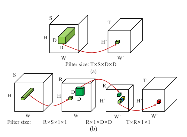
Using similar logic as defined before, the number of multiplies required for this operation in . Thus a convolution layer is simply a multiplication operation over a subset of a tensor yielding a smaller tensor. We can approximate the kernel using a series of "smaller" multiplication operations by reducing the dimensions we need to multiply across. Consider the following decomposition,

This is similar to the case of the SVD with an important difference the core is a 4 dimensional tensor and not a matrix. Where the first term in each bracket is the size and the second term is the number of multiplies. The size is of one kernel whereas the number of multiplies is the total number of multiplies to generate the complete output (i.e. if the operation denoted by the red arrows was calculated for the entire input tensor to generate the entire output tensor, it is given by the formula, product of kernel dimensions product of output tensor dimensions ). : ( , ) : (, ) : (, ) Which makes the transformation function (with number of multiplies),

The number of multiplies in this operation is which is less than if and .

In the figure above each of the red arrows indicates a one convolution operation, in figure (a) you have one fairly large filter and one convolution, whereas in the figure (b) you have 3 convolution operations using 3 smaller filters. Let’s break down the space and size savings for this. Recall, for our fully connected layers this formula was,

Rank Selection

So we are ready to go with a decomposition, all that remains is finding out the optimal rank. Again, if the rank is too low we end up with high compression but possibly low accuracy, and if the rank is too high we end up with very low compression. In embedded systems we need to be quite aggressive in compression since this can be a hard constraint on solving a problem. In our previous example, we could "locally" optimize rank but in the case of CNNs this is not possible since at the very least we would have at least one FC and one convolutional layer and we must compress both somewhat simultaneously. Brute force quickly becomes hard, as for even modest tensor combinations such as and we can end up with far too many combinations to try. Binary search is also not possible since it is not clear if simultaneously lowering both ranks lowers accuracy.

Naive Rank Selection Algorithm

The intuition is that if a layer is more sensitive to decomposition it should have higher ranks. Our algorithm is proprietary but the intuition is as follows. We start with a rank of 1 and increase the rank by 1 until the accuracy drops below a certain threshold. We then decrease the rank by 1 and continue until the accuracy drops below a certain threshold. We then take the rank that gave the highest accuracy. This is a naive algorithm and can be improved upon.