Decomposition of a Convolutional layer

In a previous post I described (in some detail) what it means to decompose a matrix multiply into a sequence of low rank matrix multiplies. We can do something similar for a tensor as well, this is somewhat less easy to see since tensors (particularly in higher dimensions) are quite hard to visualize.
Recall, the matrix formulation,

Where and are the left and right singular vectors of respectively. The idea is to approximate as a sum of outer products of and of lower rank.
Now instead of a weight matrix multiplication we have a kernel operation, where is the convolution operation. The idea is to approximate as a sum of outer products of and of lower rank.
Interestingly, you can also think about this as a matrix multiplication, by creating a Toplitz matrix version of , call it and then doing . But this comes with issues as is much much bigger than . So we just approach it as a convolution operation for now.

Convolution Operation

At the heart of it, a convolution operation takes a smaller cube subset of a “cube” of numbers (also known as the map stack) multiplies each of those numbers by a fixed set of numbers (also known as the kernel) and gives a single scalar output. Let us start with what each “slice” of the cube really represents.

Now that we have a working example of the representation, let us try to visualize what a convolution is.

A convolution operation takes a subset of the RGB image across all channels and maps it to one number (a scalar), by multiplying the cube of numbers with a fixed set of numbers (a.k.a kernel, not pictured here) and adding them together.A convolution operation multiplies each pixel in the image across all channels with a fixed number and add it all up.

Low Rank Approximation of Convolution

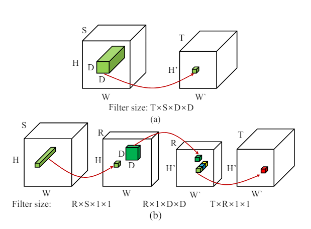
Now that we have a good idea of what a convolution looks like, we can now try to visualize what a low rank approximation to a convolution might look like. The particular kind of approximation we have chosen here does the following 4 operations to approximate the one convolution operation being done.

Painful Example of Convolution by hand

Consider the input matrix :

Input slice:

Kernel:

Element-wise multiplication and sum:

Now repeat that by moving the kernel one step over (you can in fact change this with the stride argument for convolution).

Low Rank Approximation of convolution

Now we will painfully do a low rank decomposition of the convolution kernel above. There is a theorem that says that a matrix can be approximated by a sum of 2 outer products of two vectors. Say we can express as,

We can easily guess . Consider,

This is easy because I chose values for the kernel that were easy to break down. How to perform this breakdown is the subject of the later sections.

Consider the original kernel matrix and the low-rank vectors:

The input matrix is:

Convolution with Original Kernel

Perform the convolution at the top-left corner of the input matrix:

Convolution with Low-Rank Vectors

Using the low-rank vectors:

Step 1: Apply (filter along the columns):**

Step 2: Apply (sum along the rows):**

Comparison

• Convolution with Original Kernel: -2

• Convolution with Low-Rank Vectors: 0

The results are different due to the simplifications made by the low-rank approximation. But this is part of the problem that we need to optimize for when picking low rank approximations. In practice, we will ALWAYS lose some accuracy

PyTorch Implementation

Below you can find the original definition of AlexNet.

1
2
3
4
5
6
7
8
9
10
11
12
13
14
15
16
17
18
19
20
21
22
23
24
25
26
27
28
29
30
31
32
33
34
35
36
37
38
39
40
41
42
43
44
45
46
47
48
49
50
51
52
53
54

class Net(nn.Module):
    def __init__(self):
        super().__init__()
        self.layers  = nn.ModuleDict()
        self.layers['conv1'] = nn.Conv2d(3, 6, 5)
        self.layers['pool'] = nn.MaxPool2d(2, 2)
        self.layers['conv2'] = nn.Conv2d(6, 16, 5)
        self.layers['fc1'] = nn.Linear(16 * 5 * 5, 120)
        self.layers['fc2'] = nn.Linear(120, 84)
        self.layers['fc3'] = nn.Linear(84, 10)

    def forward(self,x):
        x = self.layers['pool'](F.relu(self.layers['conv1'](x)))
        x = self.layers['pool'](F.relu(self.layers['conv2'](x)))
        x = torch.flatten(x, 1)
        x = F.relu(self.layers['fc1'](x))
        x = F.relu(self.layers['fc2'](x))
        x = self.layers['fc3'](x)
        return x

def evaluate_model(net):
    import torchvision.transforms as transforms
    batch_size = 4 # [4, 3, 32, 32]
    transform = transforms.Compose(
        [transforms.ToTensor(),
         transforms.Normalize((0.5, 0.5, 0.5), (0.5, 0.5, 0.5))])
    classes = ('plane', 'car', 'bird', 'cat',
               'deer', 'dog', 'frog', 'horse', 'ship', 'truck')
    trainset = torchvision.datasets.CIFAR10(root='../data', train=True,
                                            download=True, transform=transform)
    trainloader = torch.utils.data.DataLoader(trainset, batch_size=batch_size,
                                              shuffle=True, num_workers=2)
    testset = torchvision.datasets.CIFAR10(root='../data', train=False,
                                           download=True, transform=transform)
    testloader = torch.utils.data.DataLoader(testset, batch_size=batch_size,
                                             shuffle=False, num_workers=2)
    # prepare to count predictions for each class
    correct_pred = {classname: 0 for classname in classes}
    total_pred = {classname: 0 for classname in classes}
    # again no gradients needed
    with torch.no_grad():
        for data in testloader:
            images, labels = data
            outputs = net(images)
            _, predictions = torch.max(outputs, 1)
            # collect the correct predictions for each class
            for label, prediction in zip(labels, predictions):
                if label == prediction:
                    correct_pred[classes[label]] += 1
                total_pred[classes[label]] += 1
    # print accuracy for each class
    for classname, correct_count in correct_pred.items():
        accuracy = 100 * float(correct_count) / total_pred[classname]
        print(f'Original Accuracy for class: {classname:5s} is {accuracy:.1f} %')

Now let us decompose the first convolutional layer into 3 simpler layers using SVD

1
2
3
4
5
6
7
8
9
10
11
12
13
14
15
16
17
18
19
20
21
22
23
24
25
26
27
28
29
30
31
32
33
34
35
36
37
38
39
40
41
42
43
44
45
46
47
48
49
50
51
52
53
54
55
56
57
58
59
60
61
62
63
64
65
66
67
68
69
70
71
72
73
74
75
76
77
78
79
80
81
82
83
84
85
86
87
88
89
90
91
92
93
94
95

def slice_wise_svd(tensor,rank):
    # tensor is a 4D tensor
    # rank is the target rank
    # returns a list of 4D tensors
    # each tensor is a slice of the input tensor
    # each slice is decomposed using SVD
    # and the decomposition is used to approximate the slice
    # the approximated slice is returned as a 4D tensor
    # the list of approximated slices is returned
    num_filters, input_channels, kernel_width, kernel_height = tensor.shape
    kernel_U = torch.zeros((num_filters, input_channels,kernel_height,rank))
    kernel_S = torch.zeros((input_channels,num_filters,rank,rank))
    kernel_V = torch.zeros((num_filters,input_channels,rank,kernel_width))
    approximated_slices = []
    reconstructed_tensor = torch.zeros_like(tensor)
    for i in range(num_filters):
        for j in range(input_channels):
            U, S, V = torch.svd(tensor[i, j,:,:])
            U = U[:,:rank]
            S = S[:rank]
            V = V[:,:rank]
            kernel_U[i,j,:,:] = U
            kernel_S[j,i,:,:] = torch.diag(S)
            kernel_V[i,j,:,:] = torch.transpose(V,0,1)


    # print the reconstruction error
    print("Reconstruction error: ",torch.norm(reconstructed_tensor-tensor).item())

    return kernel_U, kernel_S, kernel_V

def svd_decomposition_conv_layer(layer, rank):
    """ Gets a conv layer and a target rank,
        returns a nn.Sequential object with the decomposition
    """

    # Perform SVD decomposition on the layer weight tensorly.
    
    layer_weight = layer.weight.data
    kernel_U, kernel_S, kernel_V = slice_wise_svd(layer_weight,rank)
    U_layer = nn.Conv2d(in_channels=kernel_U.shape[1],
                                                out_channels=kernel_U.shape[0], kernel_size=(kernel_U.shape[2], 1), padding=0, stride = 1,
                                                dilation=layer.dilation, bias=True)
    S_layer = nn.Conv2d(in_channels=kernel_S.shape[1],
                                                out_channels=kernel_S.shape[0], kernel_size=1, padding=0, stride = 1,
                                                dilation=layer.dilation, bias=False)
    V_layer = nn.Conv2d(in_channels=kernel_V.shape[1],
                                                out_channels=kernel_V.shape[0], kernel_size=(1, kernel_V.shape[3]), padding=0, stride = 1,
                                                dilation=layer.dilation, bias=False)
    # store the bias in U_layer from layer
    U_layer.bias = layer.bias

    # set weights as the svd decomposition
    U_layer.weight.data = kernel_U
    S_layer.weight.data = kernel_S
    V_layer.weight.data = kernel_V

    return [U_layer, S_layer, V_layer]
    
    
class lowRankNetSVD(Net):
    def __init__(self, original_network):
        super().__init__()
        self.layers = nn.ModuleDict()
        self.initialize_layers(original_network)
    
    def initialize_layers(self, original_network):
        # Make deep copy of the original network so that it doesn't get modified
        og_network = copy.deepcopy(original_network)
        # Getting first layer from the original network
        layer_to_replace = "conv1"
        # Remove the first layer
        for i, layer in enumerate(og_network.layers):
            if layer == layer_to_replace:
                # decompose that layer
                rank = 1
                kernel = og_network.layers[layer].weight.data
                decomp_layers = svd_decomposition_conv_layer(og_network.layers[layer], rank)
                for j, decomp_layer in enumerate(decomp_layers):
                    self.layers[layer + f"_{j}"] = decomp_layer
            else:
                self.layers[layer] = og_network.layers[layer]
    
    def forward(self, x):
        x = self.layers['conv1_0'](x)
        x = self.layers['conv1_1'](x)
        x = self.layers['conv1_2'](x)
        x = self.layers['pool'](F.relu(x))
        x = self.layers['pool'](F.relu(self.layers['conv2'](x)))
        x = torch.flatten(x, 1)
        x = F.relu(self.layers['fc1'](x))
        x = F.relu(self.layers['fc2'](x))
        x = self.layers['fc3'](x)
        return x

Decomposition into a list of simpler operations

The examples above are quite simple and are perfectly good for simplifying neural networks. This is still an active area of research. One of the things that researchers try to do is try to further simplify each already simplified operation, of course you pay the price of more operations. The one we will use for this example is one where the operations is broken down into four simpler operations.

• (Green) Takes one pixel from the image across all channels and maps it to one value

• (Red) Takes one long set of pixels from one channel and maps it to one value

• (Blue) Takes one wide set of pixels from one channel and maps it to one value

• (Green) takes one pixel from all channels and maps it to one value

Intuitively, we are still taking the subset “cube” but we have broken it down so that in any given operation only dimension is not . This is really the key to reducing the complexity of the initial convolution operation, because even though there are more such operations each operations is more complex.

PyTorch Implementation

In this section, we will take AlexNet (Net), evaluate (evaluate_model) it on some data and then decompose the convolutional layers.

Declaring both the original and low rank network

Here we will decompose the second convolutional layer, given by the layer_to_replace argument. The two important lines to pay attention to are est_rank and cp_decomposition_conv_layer. The first function estimates the rank of the convolutional layer and the second function decomposes the convolutional layer into a list of simpler operations.

1
2
3
4
5
6
7
8
9
10
11
12
13
14
15
16
17
18
19
20
21
22
23
24
25
26
27
28
29
30
31
32
33
34
35
36
37

class lowRankNet(Net):

    def __init__(self, original_network):
        super().__init__()
        self.layers = nn.ModuleDict()
        self.initialize_layers(original_network)

    def initialize_layers(self, original_network):
        # Make deep copy of the original network so that it doesn't get modified
        og_network = copy.deepcopy(original_network)
        # Getting first layer from the original network
        layer_to_replace = "conv2"
        # Remove the first layer
        for i, layer in enumerate(og_network.layers):
            if layer == layer_to_replace:
                # decompose that layer
                rank = est_rank(og_network.layers[layer])
                decomp_layers = cp_decomposition_conv_layer(og_network.layers[layer], rank)
                for j, decomp_layer in enumerate(decomp_layers):
                    self.layers[layer + f"_{j}"] = decomp_layer
            else:
                self.layers[layer] = og_network.layers[layer]
        # Add the decomposed layers at the position of the deleted layer

    def forward(self, x, layer_to_replace="conv2"):
        x = self.layers['pool'](F.relu(self.layers['conv1'](x)))
        # x = self.layers['pool'](F.relu(self.laye['conv2'](x)
        x = self.layers['conv2_0'](x)
        x = self.layers['conv2_1'](x)
        x = self.layers['conv2_2'](x)
        x = self.layers['pool'](F.relu(self.layers['conv2_3'](x)))
        x = torch.flatten(x, 1)
        x = F.relu(self.layers['fc1'](x))
        x = F.relu(self.layers['fc2'](x))
        x = self.layers['fc3'](x)
        return x

Evaluate the Model

You can evaluate the model by running the following code. This will print the accuracy of the original model and the low rank model.

1
2
3
4
5
6
7
8
9
10
11
12
13
14
15
16
17
18
19
20
21
22

decomp_alexnet = lowRankNetSVD(net)
# replicate with original model

correct_pred = {classname: 0 for classname in classes}
total_pred = {classname: 0 for classname in classes}

# again no gradients needed
with torch.no_grad():
    for data in testloader:
        images, labels = data
        outputs = decomp_alexnet(images)
        _, predictions = torch.max(outputs, 1)
        # collect the correct predictions for each class
        for label, prediction in zip(labels, predictions):
            if label == prediction:
                correct_pred[classes[label]] += 1
            total_pred[classes[label]] += 1

# print accuracy for each class
for classname, correct_count in correct_pred.items():
    accuracy = 100 * float(correct_count) / total_pred[classname]
    print(f'Lite Accuracy for class: {classname:5s} is {accuracy:.1f} %')

Let us first discuss estimate rank. For a complete discussion see the the references by Nakajima and Shinchi. The basic idea is that we take the tensor, “unfold” it along one axis (basically reduce the tensor into a matrix by collapsing around other axes) and estimate the rank of that matrix.
You can find est_rank below.

1
2
3
4
5
6
7
8
9
10
11
12
13
14
15
16
17
18
19
20
21
22
23
24
25
26
27
28
29
30
31
32
33
34
35
36
37
38
39
40
41
42
43
44
45
46
47
48
49
50
51
52
53
54
55
56
57
58
59
60
61
62
63
64
65
66
67
68
69
70
71
72
73
74
75
76
77
78
79
80
81
82
83
84
85
86
87
88
89
90
91
92
93
94
95
96
97
98
99
100
101
102
103
104
105
106
107
108
109
110
111
112
113
114

from __future__ import division
import torch
import numpy as np
# from scipy.sparse.linalg import svds
from scipy.optimize import minimize_scalar
import tensorly as tl

def est_rank(layer):
    W = layer.weight.data
    # W = W.detach().numpy() #the weight has to be a numpy array for tl but needs to be a torch tensor for EVBMF
    mode3 = tl.base.unfold(W.detach().numpy(), 0)
    mode4 = tl.base.unfold(W.detach().numpy(), 1)
    diag_0 = EVBMF(torch.tensor(mode3))
    diag_1 = EVBMF(torch.tensor(mode4))

    # round to multiples of 16
    multiples_of = 8 # this is done mostly to standardize the rank to a standard set of numbers, so that 
    # you do not end up with ranks 7, 9 etc. those would both be approximated to 8.
    # that way you get a sense of the magnitude of ranks across multiple runs and neural networks
    # return int(np.ceil(max([diag_0.shape[0], diag_1.shape[0]]) / 16) * 16)
    return int(np.ceil(max([diag_0.shape[0], diag_1.shape[0]]) / multiples_of) * multiples_of)

def EVBMF(Y, sigma2=None, H=None):
    """Implementation of the analytical solution to Empirical Variational Bayes Matrix Factorization.
    This function can be used to calculate the analytical solution to empirical VBMF.
    This is based on the paper and MatLab code by Nakajima et al.:
    "Global analytic solution of fully-observed variational Bayesian matrix factorization."

    Notes
    -----
        If sigma2 is unspecified, it is estimated by minimizing the free energy.
        If H is unspecified, it is set to the smallest of the sides of the input Y.

    Attributes
    ----------
    Y : numpy-array
        Input matrix that is to be factorized. Y has shape (L,M), where L<=M.

    sigma2 : int or None (default=None)
        Variance of the noise on Y.

    H : int or None (default = None)
        Maximum rank of the factorized matrices.

    Returns
    -------
    U : numpy-array
        Left-singular vectors.

    S : numpy-array
        Diagonal matrix of singular values.

    V : numpy-array
        Right-singular vectors.

    post : dictionary
        Dictionary containing the computed posterior values.


    References
    ----------
    .. [1] Nakajima, Shinichi, et al. "Global analytic solution of fully-observed variational Bayesian matrix factorization." Journal of Machine Learning Research 14.Jan (2013): 1-37.

    .. [2] Nakajima, Shinichi, et al. "Perfect dimensionality recovery by variational Bayesian PCA." Advances in Neural Information Processing Systems. 2012.
    """
    L, M = Y.shape  # has to be L<=M

    if H is None:
        H = L

    alpha = L / M
    tauubar = 2.5129 * np.sqrt(alpha)

    # SVD of the input matrix, max rank of H
    U, s, V = torch.svd(Y)
    U = U[:, :H]
    s = s[:H]
    V[:H].t_()

    # Calculate residual
    residual = 0.
    if H < L:
        residual = torch.sum(torch.sum(Y ** 2) - torch.sum(s ** 2))

    # Estimation of the variance when sigma2 is unspecified
    if sigma2 is None:
        xubar = (1 + tauubar) * (1 + alpha / tauubar)
        eH_ub = int(np.min([np.ceil(L / (1 + alpha)) - 1, H])) - 1
        upper_bound = (torch.sum(s ** 2) + residual) / (L * M)
        lower_bound = np.max([s[eH_ub + 1] ** 2 / (M * xubar), torch.mean(s[eH_ub + 1:] ** 2) / M])

        scale = 1.  # /lower_bound
        s = s * np.sqrt(scale)
        residual = residual * scale
        lower_bound = float(lower_bound * scale)
        upper_bound = float(upper_bound * scale)

        sigma2_opt = minimize_scalar(EVBsigma2, args=(L, M, s, residual, xubar), bounds=[lower_bound, upper_bound],
                                     method='Bounded')
        sigma2 = sigma2_opt.x

    # Threshold gamma term
    threshold = np.sqrt(M * sigma2 * (1 + tauubar) * (1 + alpha / tauubar))

    pos = torch.sum(s > threshold)
    if pos == 0: return np.array([])

    # Formula (15) from [2]
    d = torch.mul(s[:pos] / 2,
                  1 - (L + M) * sigma2 / s[:pos] ** 2 + torch.sqrt(
                      (1 - ((L + M) * sigma2) / s[:pos] ** 2) ** 2 - \
                      (4 * L * M * sigma2 ** 2) / s[:pos] ** 4))

    return torch.diag(d)

You can find the EVBMF code on my github page. I do not go into it in detail here. Jacob Gildenblatt’s code is a great resource for an in-depth look at this algorithm.

Conclusion

So why is all this needed? The main reason is that we can reduce the number of operations needed to perform a convolution. This is particularly important in embedded systems where the number of operations is a hard constraint. The other reason is that we can reduce the number of parameters in a neural network, which can help with overfitting. The final reason is that we can reduce the amount of memory needed to store the neural network. This is particularly important in mobile devices where memory is a hard constraint.
What does this mean mathematically? Fundamentally it means that neural networks are over parameterized i.e. they have far more parameters than the information that they represent. By reducing the rank of the matrices needed carry out a convolution, we are representing the same operation (as closely as possible) with a lot less information.

References

• [Low Rank approximation of CNNs] (https://arxiv.org/pdf/1511.06067)
• [CP Decomposition] (https://arxiv.org/pdf/1412.6553)
• Kolda & Bader “Tensor Decompositions and Applications”in SIAM REVIEW, 2009
• [1] Nakajima, Shinichi, et al. “Global analytic solution of fully-observed variational Bayesian matrix factorization.” Journal of Machine Learning Research 14.Jan (2013): 1-37.
• [2] Nakajima, Shinichi, et al. “Perfect dimensionality recovery by variational Bayesian PCA.”
• [Python implementation of EVBMF] (https://github.com/CasvandenBogaard/VBMF)
• [Accelerating Deep Neural Networks with Tensor Decompositions - Jacob Gildenblat] (https://jacobgil.github.io/deeplearning/tensor-decompositions-deep-learning)
• [Python Implementatioon of VBMF] (https://github.com/CasvandenBogaard/VBMF)
• [Similar article that is more high level] (https://medium.com/@anishhilary97/low-rank-approximation-for-4d-kernels-in-convolutional-neural-networks-through-svd-65b30dc55f6b)

Introduction

A common question I had when I first started working with quantization was, how exactly are values passed between layers post quantization? Looking at the quantization equations it was not immediately obvious to me how to do away with ALL floating point operations and what values were used exactly in the forward pass operation.
In this article, I will address two main questions,

• How does PyTorch pass values between layers post quantization? And what are the quantization equations used.
• What exactly makes floating point operations slower than integer operations?

In short, PyTorch passes integer values between layers when in INT8 only quantization. It does so using a few neat tricks of fixed point and floating point math. When in other quantization modes, values passed between layers can be float.

Quantized Matrix Multiplication

The overall goal of quantization is to make this multiplication operation simpler in some sense, There are two ways to make this simpler,

• Carry out the multiplication operation in integers, as of now are floats

• save as an integers

We can achieve both ends by,

• replacing by

• adding subtracting terms to get back the original value

We can use the well known quantization scheme to carry out the quantization for each of these objects. As a recap, they are outlined again below. Personally, I just took these functions as given and “magically” converted between integers and floats, it is not quite that important to understand their inner workings at this stage. Using the quantization scheme, and de-quantization scheme,

We can write the above multiplication as, Notice that now, instead of multiplying we have an expression where we eventually we get the integer multiply . In fact, is also an integer multiply so we can leave it at that stage instead. Notice that is still float, thus, Thus, we can write, Notice that, each of the matrix multiplies are integers, but the preceding coefficients are floats. This is a problem, since if our embedded system only supports integer multiplies we will not be able to do this operation. Notice also that bias’ quantization prevents us from efficiently doing the operation in one step without a multiply in between. We will solve this second issue first, Notice that instead of choosing the scale and range “correctly" we can choose them somewhat arbitrarily as long as they work. In particular we can choose to quantize such that and . This usually under-quantizes the bias, but its good for two reasons,

• Bias tends to be more important for accuracy than weights do, so it is in fact better if its higher in accuracy

• Even though they are bigger than they need to be they account for a fraction of the parameters of the neural network.

For the first issue, we use a pretty neat trick. Remember that is constant and we know it at the time of compiling, so we can consider it to be a fixed point operation, we can write it as where is always a fixed number determined at the time of compilation (this is not true for floating point). Thus the entire expression, can be carried out with integer arithmetic and all values exchanged between layers are integer values.

Data Types Passed Between Layers

Using the matrix multiplication example before, are the weights and biases of one fully connected layer. A question I often had was, how exactly are values passed between layers. This is because FULL INT8 quantization essentially means you can deploy a neural network on a board that does not support ANY floating point operations. It is in fact the that is passed between layers when you do INT8 quantization. However, if you just need the weights and the multiplies to be quantized but not the activations, it means that you are getting the benefits of quantization for saving space of the weights and by using integer multiply BUT are choosing to pass values between the layers as floats. For this case, PyTorch and Keras can also spit out the floating point values, to be passed between layers, and it does this by simply omitting the de-quantization step. Here again, we can choose but I am not sure if this additional assumption is needed, since the board has the ability to do floating point multiplications it does not matter if one or more float multiplies are needed.

To summarize,

• For full INT8 quantization i.e. when the embedded device does not support any floating point multiplies use

• For partial INT8 quantization i.e. you want the activations to be in float but weights and integer multiplies to be done in/ saved as INT8 use the equation for .

Why Exactly Does Floating Point Slow Things Down?

Another paint point for me was the lack of reasoning as to why multiplying two floating point numbers together takes longer/ is more difficult than multiplying two INTs together. The reason has to do with physics, and we will come to it in a minute. For now let us consider two floating point numbers and their resulting multiplication. Recall, that a floating point number is always of the form . Where the leading is compulsory, if any calculation results in values such as , you need to divide the mantissa by and keep adding it to the exponent. Additionally, means that you can only store values past the radix point (general word for what the point ‘’ is binary system).

Consider, and

• Add, the exponents

• Multiply, the mantissas

• Re-normalize, by dividing by , exponent is now , mantissa is 1.00011

• Sign, here both numbers are positive so the sign bit is

• Truncate,

As you can see, multiplying two floating point numbers takes quite a bit of steps. In particular, re-normalization could potentially take multiple steps.

For contrast, consider a fixed point multiplication, and . In this case is forced to use , so in memory this step is simply omitted. For multiplication is automatically assumed.

• Add, exponents

• Multiply, the mantissas 0.100011

• Re-normalize,

• Sign, here both numbers are positive so the sign bit is

Even though the re-normalization stage seems the same, it is actually always the same number of steps, whereas for the floating point case it can be arbitrarily long and needs to check whether there is a leading .
pandoc version 3.2

Conclusion

In this article, we discussed how values are passed between layers post quantization in PyTorch. We also discussed why floating point operations are slower than integer operations. I hope this article was helpful in understanding the inner workings of quantization and the differences between floating point and integer operations. Again, PyTorch makes things very simple by doing things for you but if you need to understand the underlying concepts then you need to open things up and verify.

References

https://arxiv.org/pdf/1712.05877
https://arxiv.org/pdf/1806.08342

Introduction

The packaging of extremely complex techniques inside convenient wrappers in PyTorch often makes quick implementations fairly easy, it also removes the need to understand the inner workings of the code. However, this obfuscates the theory of why such things work and why they are important to us. For instance, for neither love or money, could I figure out what a QuantStub and a DeQuant Stub really do and how to replicate that using pen and paper. In embedded systems one often has to code up certain things from scratch, as it were and sometimes PyTorch’s “convenience” can be a major impediment to understanding the underlying theory. In the code below, I will show you how to quantize a single layer of a neural network using PyTorch. And explain each step in excruciating detail. At the end of this article you will be able to implement quantization in PyTorch (or indeed any other library) but crucially, you will be able to do it without using any quantize layers, you can essentially use the usual “vanilla” layers. But before that we need to understand how or why quantization is important.

Quantization

The process of quantization is the process of reducing the number of bits that represent a number. This usually means we want to use an integer instead of a real number, that is, you want to go from using a floating point number to an integer. It is important to note that the reason for this is because of the way we multiply numbers in embedded systems. This has to do with both the physics and the chemistry of a half-adder and a full adder. It just takes longer to multiply two floats together than it does to multiply two integers together. For instance, multiplying is a much more complex operation than multiplying . So it is not simply a consequence of reducing the “size” of the number. In the future, I will write a blog post about why physics has a lot to do with why this is.

Outline

I start with the intuition behind Quantization using a helpful example. And then I outline a manual implementation of quantization in PyTorch. So what exactly does “manual” mean?

1. I will take a given, assumed pre-trained, PyTorch model (1 Fully connected layer with no bias) that has been quantized using PyTorch’s quantization API.
2. I will extract the weights of the layer and quantize them manually using the scale and zero point from the PyTorch quantization API.
3. I will quantize the input to the layer manually, using the same scale and zero point as the PyTorch quantization API.
4. I will construct a “vanilla” fully connected layer (as opposed to the quantized layer in step 1) and multiply the quantized weights and input to get the output.
5. I will compare the output of the quantized layer from step 1 with the output of the “vanilla” layer from step 4.

This will inherently allow you to understand the following :

1. How to quantize a layer in PyTorch and what quantizing in PyTorch really means.
2. Some potentially confusing issues about what is being quantized, how and why.
3. What does the QuantStub and DeQuantStub really do and how to replicate that using pen and paper.

At the end of this article you should be able to :

1. Understand Quantization conceptually.
2. Understand PyTorch’s quantization API.
3. Implement quantization manually in PyTorch.
4. Implement a Quantized Neural Network in PyTorch without using PyTorch’s quantization API.

Intuition behind Quantization

The best way to think about quantization is to think of it through an example. Let’s say you own a store, and you are printing labels for the prices of objects, but you want to economize on the number of labels you print. Assume here for simplicity that you can print a label that shows a price lower than the price of the product but not more. If you print tags for 0.20 cents, you get the following table, which shows a loss of 0.97 by printing 6 labels. This obviously didn’t save you much as you might as well have printed labels with the original prices and lost in sales.

Maybe we can be more aggressive, by choosing tags rounded to the nearest dollar instead, we can obviously lose more money but we save on one whole tag!

How about an even more aggressive one? We round to the nearest dollars and use just two tags. But then we are stuck with a massive loss of dollars.

In this example, the price tags represent memory units and each price tag printed costs a certain amount of memory. Obviously, printing as many price tags as there are goods results in no loss of money but also the worst possible outcome as far as memory is concerned. Going the other way reducing the number of tags results in the largest loss in money.

Quantization as an (Unbounded) Optimization Problem

Clearly, this calls for an optimization problem, so we can set up the following one : let be the quantization function , then the loss is as follows,

Where is a count of the unique values that over the entire interval of, .

Issues with finding a solution

A popular assumption is to assume that the function is a rounding of a linear transformation. The constraint that minimizes is difficult since the function is unbounded. We could solve this if we knew at least two points at which we knew the expected output for the quantization problem, but we do not, since there is no bound on the highest tag we can print. If we could impose a bound on the problem, we could evaluate the function at the two bounds and solve it. Thus setting a bound seems to solve both problems.

Quantization as Bounded Optimization Problem

In the previous section, our goal was to reduce the number of price tags we print, but it was not a bounded problem. In your average grocery story prices could run between dollars and a dollars. Using the scheme above you could certainly print fewer labels. But you could also end up printing a large number of labels in absolute terms. You could do one better by pre-determining the number of labels you want to print. Let us then, set some bounds on the number of labels we want to print, consider the labels you want to print as , this is fairly aggressive. Again we can set up the optimization problem as follows (there is no need to minimze , the count of unique labels for now, since we are defining that ourselves), where is the scale and is the zero point. It must be true that, Evaluating the above equations gives us the general solution This gives us the solution, .

This gives the oft quoted quantization formula, Similarly, we get reverse the formula to get the dequantization formula i.e. starting from a quantized value we can guess what the original value must have been, This is obviously lossy.

Implication of Quantization

We have shown that given some prices, we can quantize them to a smaller set of labels. Thus saving on the cost of labels. What if you remembered and and then you used the dequantization formula to guess what the original price was and charge the customer that amount? This way you can save on the number of labels, but you can get closer to the original price by just writing down and and using the dequantization formula. We can actually do a better job with prices as well as saving on the number of labels. However, this is lossy, and you will lose some money. In this example, we notice that we consider charging more or less than the actual price as a loss both ways, to keep things simple.

Quantization of Matrix Multiplication

Using this we can create a recipe for quantization to help us in the case of neural networks. Recall that the basic unit of a neural network is the operation,

We can apply quantization to the weights and the input (). We can then use dequantization to get the output.

Our goal of trying to avoid the floating point multiplication between can now be achieved by replacing them with their respective quantized values and scaling and subtracting the zero point to get the final output. Here, and are quantized matrices and thus the multiplication operation (after multiplying it out) is now not between two floating point matrices and but between and . Which are both integer matrices. This allows us to save on memory and computation since it is cheaper to multiply integers together than it is to multiple floats. However, in practice since, are also integers, is also an integer multiplication, so we just use that mulitplication instead of multiplying out the whole thing.

Code

Consider the following original,

1
2
3
4
5
6
7
8
9
10
11
12
13
14
15
16
17
18

class M(torch.nn.Module):
    def __init__(self):
        super(M, self).__init__()
        # QuantStub converts tensors from floating point to quantized
        self.quant = torch.quantization.QuantStub()
        self.fc = torch.nn.Linear(2, 2, bias=False)
        # DeQuantStub converts tensors from quantized to floating point
        self.dequant = torch.quantization.DeQuantStub()

    def forward(self, X):
        # manually specify where tensors will be converted from floating
        # point to quantized in the quantized model
        X = self.quant(X)
        x = self.fc(X) # [[124.,  36.]
        # manually specify where tensors will be converted from quantized
        # to floating point in the quantized model
        x = self.dequant(x)
        return x

Now consider, the manual quantization of the weights and the input. model_int8 represents the quantized model. The QuantM2 class is the manual quantization of the model. The prepare_model function uses PyTorch convenience functions for quantization of the weights and the input i.e. get , from this model and compute the other steps. You can calculate these yourself as well, using the distributions of the input data and activation functions. The quantize_tensor_unsigned function is the manual quantization of the input tensor. The pytorch_result function is that computes the output of the fully connected layer of the PyTorch quantized model. The forward function is the manual quantization of the forward pass of the model.

1
2
3
4
5
6
7
8
9
10
11
12
13
14
15
16
17
18
19
20
21
22
23
24
25
26
27
28
29
30
31
32
33
34
35
36
37
38
39
40
41
42
43
44
45
46
47
48
49
50
51
52
53
54
55
56
57
58
59
60
61
62

def prepare_model(model_fp32, input_fp32):
    # model must be set to eval mode for static quantization logic to work
    model_fp32.eval()
    model_fp32.qconfig = torch.quantization.QConfig(
        activation=MinMaxObserver.with_args(dtype=torch.quint8),
        weight=MinMaxObserver.with_args(dtype=torch.qint8)
    )
    # Prepare the model for static quantization. This inserts observers in
    # the model that will observe activation tensors during calibration.
    model_fp32_prepared = torch.quantization.prepare(model_fp32)
    model_fp32_prepared(input_fp32)

    model_int8 = torch.quantization.convert(model_fp32_prepared)
    return model_int8


def quantize_tensor_unsigned(x, scale, zero_point, num_bits=8):
    # This function mocks the PyTorch QuantStub function which quantizes the input tensor
    qmin = 0.
    qmax = 2. ** num_bits - 1.

    q_x = zero_point + x / scale
    q_x.clamp_(qmin, qmax).round_()
    q_x = q_x.round().byte()

    return QTensor(tensor=q_x, scale=scale, zero_point=zero_point)
    
class QuantM2(torch.nn.Module):

    def __init__(self, model_fp32, input_fp32):
        super(QuantM2, self).__init__()
        self.fc = torch.nn.Linear(2, 2, bias=False)
        self.model_int8 = prepare_model(model_fp32, input_fp32)
        # PyTorch automatically quantizes the model for you, we will use those weights to compute a forward pass
        W_q = self.model_int8.fc.weight().int_repr().double() 
        z_w = self.model_int8.fc.weight().q_zero_point()
        self.fc.weight.data = (W_q - z_w)

    @staticmethod
    def pytorch_result(model_int8, input_fp32):
        pytorch_res = model_int8.fc(model_int8.quant(input_fp32)).int_repr().float()
        return pytorch_res

    def forward(self, x):
            input_fp32 = x
            s_x = self.model_int8.quant(input_fp32).q_scale()
            z_x = self.model_int8.quant(input_fp32).q_zero_point()
            quant_input_unsigned = quantize_tensor_unsigned(input_fp32, s_x,z_x)
            z_x = quant_input_unsigned.zero_point
            s_x = quant_input_unsigned.scale
            s_w = self.model_int8.fc.weight().q_scale()
            x1 = self.fc(quant_input_unsigned.tensor.double() - z_x)
            # this next step is equivalent to dequantizing the output of the fully connected layer
            # it not exactly equivalent since I already subtracted the two zero points
            # you can derive a much longer quantization formula that multiplies W_q * X_q and has additional terms
            # you can then put W_q in the fc layer and X_q in the forward pass
            # and then use all those additional terms in the below step to requantize
            # in embedded systems its easy to use the formulation here
            x1 = x1 * (s_x * s_w)
            return x1

Sample run code of the above code is as follows,

1
2
3
4
5
6
7
8
9

cal_dat = torch.randn(1, 2)
model = M()
# graph mode implementation
sample_data = torch.randn(1, 2)
model(sample_data)
quant_model= QuantM2(model_fp32=model, input_fp32=sample_data)
quant_model(sample_data)
quant_model.model_int8(sample_data) # this is the quantized model, M2 should match it exactly, M is the original non quantized model. For small data sets there is usually no divergence.
# but in practice, the quantized model will be faster and use less memory, but will lose some accuracy

Let us start by analyzing the output of a quant layer of our simple model. The output of the int_models quantized layer is (somewhat counter-intuitively) always a float, this does not mean it is not quantized, it simply means you are shown the non-quantized value. If you look at the output, you will notice, it has dtype, quantization_scheme, scale and zero_point. You can view the value that will actually be used when it is called within the context of a quant layer by calling its int representation.

1
2
3
4
5
6
7
8
9
10
11
12

#recreate quant layer
int_model = quant_model.model_int8
default_pytorch_quant_layer_output = int_model.quant(sample_data)
# OUTPUT
# tensor([[0.1916, 0.5428]], size=(1, 2), dtype=torch.quint8,
#        quantization_scheme=torch.per_tensor_affine, scale=0.0021285151597112417,
#        zero_point=0)

actual_pytorch_quant_layer_output = int_model.quant(sample_data).int_repr()
# OUTPUT
# tensor([[90, 255]], dtype=torch.uint8)

Our manual quantization layer is a bit different, it outputs a QTensor object, which contains the tensor, the scale and the zero point. We get the scale and the zero point from the PyTorch quantized model’s quant layer (again, we could easily have done this by ourselves using the sample data).

1
2
3

manual_quant_layer_output = quantize_tensor_unsigned(sample_data, int_model.quant(sample_data).q_scale(), int_model.quant(sample_data).q_zero_point())
# OUTPUT
# QTensor(tensor=tensor([[ 90, 255]], dtype=torch.uint8), scale=0.0021285151597112417, zero_point=0)

Now let us look at the output of the quant layer AND the fully connected layer.

1
2
3
4
5

#recreate the fully connected layer operation
pytorch_fc_quant_layer_output = int_model.dequant(int_model.fc(int_model.quant(sample_data)))
# tensor([[-0.7907,  0.6919]])
manual_fc_quant_layer_output = quant_model(sample_data)
# tensor([[-0.7886,  0.6932]], dtype=torch.float64, grad_fn=<MulBackward0>)

It is worthwhile to point out a few things. First, the following two commands seem to give the same values but are very different. The first is a complete tensor object that gives float values but is actually quantized, look at dtype, it is actually quint.8.

1
2
3
4

int_model.fc(int_model.quant(sample_data))
# tensor([[-0.7907,  0.6919]], size=(1, 2), dtype=torch.quint8,
#        quantization_scheme=torch.per_tensor_affine, scale=0.0058139534667134285,
#        zero_point=136)

The output of this is a truly a float tensor, it not only shows as float values (same as before) but contains no quantization information.

1
2

int_model.dequant(int_model.fc(int_model.quant(sample_data)))
 # tensor([[-0.7907,  0.6919]])

Thus, in order to recreate a quantization operation from PyTorch in any embedded system you do not need to implement a de-quant layer. You can simply multiply and subtract zero points from your weight layers appropriately. Look for the long note inside the forward pass of the manually quantized model for more information.

A Word on PyTorch and Quantization

PyTorch’s display in the console is not always indicative of what is happening in the back end, this section should clear up some questions, you may have (since I had them). The fundamental unit of data that goes between layers in PyTorch is always a Tensor, that is always displayed as a float. This is fairly confusing since when we think of a vector/tensor as quantized we see all the data as integers. But PyTorch works differently, when a tensor is quantized it is still displayed as a float, but its quantized data type and quantization scheme to get to that data type is stored as additional attributes to the tensor object. Thus, do not be confused if you still see float values displayed, you must look at the dtype to get a clear understanding of what the values are. In order to view a quantized tensor as a int, you need to call int_repr() on the tensor object. Note, this throws an error if the tensor has not been quantized in the first place. Also, note that when PyTorch encounters a quantized tensor, it will carry out multiplication on the quantized values automatically and thus the benefits of quantization will be realized even if you do not actually see them. When exporting the model this information is packaged as well, no need for anything extra to be done.

A Word on Quant and DeQuant Stubs

This is perhaps the most confusing of all things about quantization in PyTorch, the QuantStub and DeQuantStub.

1. The job of de-quantizing something is automatically taken care of by the previous layer, as mentioned above. Thus when you come to a DeQuant Layer all it seems to do is just strip away the memory of having ever been quantized and ensures that the floating point representation is used. That is what is meant by the statement “DeQuantStub is stateless”, it literally needs nothing to function, all the information it needs to function will be packaged with the input tensor you feed into it.
2. The Quant Stub, on the other hand, is stateful it needs to know the scale and the zero point of what is being fed into it, and the network has no knowledge of the input data, which is why you need to feed data into the Neural Network to get this going, if you knew the scale and zero point of your data already you could directly input that information into the QuantStub.
3. The QuantStub and DeQuantStub are not actually layers, they are just functions that are called when the model is quantized.
4. Another huge misconception is when and where to call these layers, every example on the PyTorch repo will have the Quant and DeQuant stub sandwiching the entire network, this leads people to think that the entire network is quantized. This is not true see the following section for more information.

Do you need to insert a Quant and DeQuant Stub after every layer in your model?

Unless you know exactly what you are doing, then YES you do. In most cases, especially for first time users, you usually want to dequantize immediately after quantizing. If you want to “quantize” every multiplication operation but dequantize the result (i.e. try to bring it back to your original scale of data) then yes, you do. The Quant and DeQuant Stub is “dumb” in the sense that it does not know what the previous layer was, if you feed it a quantized tensor it dequantizes it. It has no view of your network as a whole and does not modify the behavior of the network as a whole. Recall the mathematics of what we are trying to do. We want to replace a matrix multiplication, with . Now what if you want to replace this across multiple layers i.e. you want to quantize the following expression :

Your first layer weights are and the second layer weights are . You want to quantize the entire expression. Ask yourself what do you really want to do, in most cases what you really want to do, is quantize the two matrix multiplies, you inevitably have to do, so that they do not occur in float representation but rather occur in integer. This means you want to replace with and thus replacing the whole expression with . If you do not dequantize after every layer you will end up executing the following equation, as the entire first layer will be quantized, its output will be recorded and then that quantized value in int8 will flow to the next layer. After this, all the quantization information will be lost i.e. the scale and zero point will be lost. The DeQuant layer will simply use the information from the previous layer to dequantize the output, so only the most recent layers output will be dequantized.

When do you not need to put Quant and DeQuant Stubs after every layer?

Dequantizing comes with a cost, you need to compute floating point multiplications, in order to multiply the weights with the matrix. This is certainly less than the floating point operations from the original matrix multiplication itself (a lot less than storing the output from another whole floating point matrix), but it is still a lot. However, in many of my use cases, I could get away with not dequantizing. While the real reasons are still not clear to me (like most things in neural networks), I would guess that for some of my layers the weights were not that important to getting my overall accuracy. I was also in the Quantize Aware Framework, maybe I will do a post about this too.

Conclusion

In this blog post we covered some important details about PyTorch’s implementation of quantization that are not immediately obvious. We then went on to manually implement a quantized layer and a quantized model. We then showed how to use the quantized layer and the quantized model to get the same results as the PyTorch quantized model. We also showed that the PyTorch quantized model is not actually quantized in the sense that the values are integers, but that the values are quantized in the sense that the values are stored as tensor objects (that store their quantization parameters with them) and the operations are carried out on the integers. This is a very important distinction to make. Additionally, in inference mode, you can just take out the quantized weights, and skip the fc layer step as well, you can just multiply the two matrices together. This is what I will be doing in the embedded system case. In my next posts, I will show you how to quantize a model and the physics behind why multiplying two floats is more expensive than multiplying a two integers.

Code Follow Along

The code can be found in the same tensor rank repository :
https://github.com/FranciscoRMendes/tensor-rank/blob/main/CNN_Decomposition.ipynb

Convolutional Layer Case

The primary difference between the fully connected layer case and the convolutional layer case is the fact that the convolutional kernel is a tensor. We say that the number of multiplications in an operation depends on the size of the dimensions of the tensors involved in the multiplication. It becomes critical to approximate one large multi-dimensional kernel with multiple smaller kernels of lower dimension.

Working Example

A convolution operation maps a tensor from one dimension to a tensor of another (possibly) lower dimension. If we consider an input tensor of size then a convolution layer will map this to a tensor, of size using a kernel tensor, of size .

Using similar logic as defined before, the number of multiplies required for this operation in . Thus a convolution layer is simply a multiplication operation over a subset of a tensor yielding a smaller tensor. We can approximate the kernel using a series of "smaller" multiplication operations by reducing the dimensions we need to multiply across. Consider the following decomposition,

This is similar to the case of the SVD with an important difference the core is a 4 dimensional tensor and not a matrix. Where the first term in each bracket is the size and the second term is the number of multiplies. The size is of one kernel whereas the number of multiplies is the total number of multiplies to generate the complete output (i.e. if the operation denoted by the red arrows was calculated for the entire input tensor to generate the entire output tensor, it is given by the formula, product of kernel dimensions product of output tensor dimensions ). : ( , ) : (, ) : (, ) Which makes the transformation function (with number of multiplies),

The number of multiplies in this operation is which is less than if and .

In the figure above each of the red arrows indicates a one convolution operation, in figure (a) you have one fairly large filter and one convolution, whereas in the figure (b) you have 3 convolution operations using 3 smaller filters. Let’s break down the space and size savings for this. Recall, for our fully connected layers this formula was,

Rank Selection

So we are ready to go with a decomposition, all that remains is finding out the optimal rank. Again, if the rank is too low we end up with high compression but possibly low accuracy, and if the rank is too high we end up with very low compression. In embedded systems we need to be quite aggressive in compression since this can be a hard constraint on solving a problem. In our previous example, we could "locally" optimize rank but in the case of CNNs this is not possible since at the very least we would have at least one FC and one convolutional layer and we must compress both somewhat simultaneously. Brute force quickly becomes hard, as for even modest tensor combinations such as and we can end up with far too many combinations to try. Binary search is also not possible since it is not clear if simultaneously lowering both ranks lowers accuracy.

Naive Rank Selection Algorithm

The intuition is that if a layer is more sensitive to decomposition it should have higher ranks. Our algorithm is proprietary but the intuition is as follows. We start with a rank of 1 and increase the rank by 1 until the accuracy drops below a certain threshold. We then decrease the rank by 1 and continue until the accuracy drops below a certain threshold. We then take the rank that gave the highest accuracy. This is a naive algorithm and can be improved upon.

Motivation

As someone who implements deep learning models on embedded systems, an important consideration is often the size of the model.
There are several notions of size, but the two major ones are :

• Number of elements to save, usually in the form of a matrix or tensor.
• Number of operations to perform, usually in the form of a matrix multiplication.
  The first affects the amount of memory required to store the model, while the second affects the amount of computation required to run the model.

I have worked extensively in matrix factorization before, mostly factorizing sparse matrices for recommendation systems.
Unfortunately, while there are many LoRA walk throughs using code, I was not able to find a simple succint explanation of the problem and the solution. And why it works. This article aims to address that gap by providing an elementary explanation of the problem, how to set up the optimization problem and how to solve it, in possibly linear time.
This is part I, that deals with factorizing a fully connected layer. Part II will deal with factorizing a convolutional layer.

Code Follow Along

The Jupyter Notebook for this is at https://github.com/FranciscoRMendes/tensor-rank

Introduction to Matrices

First we start with basic definitions of matrices and tensors.
If you are reading this article you probably know what a matrix is, but here is one anyway.