Decomposition of a Convolutional layer

In a previous post I described (in some detail) what it means to decompose a matrix multiply into a sequence of low rank matrix multiplies. We can do something similar for a tensor as well, this is somewhat less easy to see since tensors (particularly in higher dimensions) are quite hard to visualize.
Recall, the matrix formulation,

Where and are the left and right singular vectors of respectively. The idea is to approximate as a sum of outer products of and of lower rank.
Now instead of a weight matrix multiplication we have a kernel operation, where is the convolution operation. The idea is to approximate as a sum of outer products of and of lower rank.
Interestingly, you can also think about this as a matrix multiplication, by creating a Toplitz matrix version of , call it and then doing . But this comes with issues as is much much bigger than . So we just approach it as a convolution operation for now.

Convolution Operation

At the heart of it, a convolution operation takes a smaller cube subset of a “cube” of numbers (also known as the map stack) multiplies each of those numbers by a fixed set of numbers (also known as the kernel) and gives a single scalar output. Let us start with what each “slice” of the cube really represents.

Now that we have a working example of the representation, let us try to visualize what a convolution is.

A convolution operation takes a subset of the RGB image across all channels and maps it to one number (a scalar), by multiplying the cube of numbers with a fixed set of numbers (a.k.a kernel, not pictured here) and adding them together.A convolution operation multiplies each pixel in the image across all channels with a fixed number and add it all up.

Low Rank Approximation of Convolution

Now that we have a good idea of what a convolution looks like, we can now try to visualize what a low rank approximation to a convolution might look like. The particular kind of approximation we have chosen here does the following 4 operations to approximate the one convolution operation being done.

Painful Example of Convolution by hand

Consider the input matrix :

Input slice:

Kernel:

Element-wise multiplication and sum:

Now repeat that by moving the kernel one step over (you can in fact change this with the stride argument for convolution).

Low Rank Approximation of convolution

Now we will painfully do a low rank decomposition of the convolution kernel above. There is a theorem that says that a matrix can be approximated by a sum of 2 outer products of two vectors. Say we can express as,

We can easily guess . Consider,

This is easy because I chose values for the kernel that were easy to break down. How to perform this breakdown is the subject of the later sections.

Consider the original kernel matrix and the low-rank vectors:

The input matrix is:

Convolution with Original Kernel

Perform the convolution at the top-left corner of the input matrix:

Convolution with Low-Rank Vectors

Using the low-rank vectors:

Step 1: Apply (filter along the columns):**

Step 2: Apply (sum along the rows):**

Comparison

• Convolution with Original Kernel: -2

• Convolution with Low-Rank Vectors: 0

The results are different due to the simplifications made by the low-rank approximation. But this is part of the problem that we need to optimize for when picking low rank approximations. In practice, we will ALWAYS lose some accuracy

PyTorch Implementation

Below you can find the original definition of AlexNet.

1
2
3
4
5
6
7
8
9
10
11
12
13
14
15
16
17
18
19
20
21
22
23
24
25
26
27
28
29
30
31
32
33
34
35
36
37
38
39
40
41
42
43
44
45
46
47
48
49
50
51
52
53
54

class Net(nn.Module):
    def __init__(self):
        super().__init__()
        self.layers  = nn.ModuleDict()
        self.layers['conv1'] = nn.Conv2d(3, 6, 5)
        self.layers['pool'] = nn.MaxPool2d(2, 2)
        self.layers['conv2'] = nn.Conv2d(6, 16, 5)
        self.layers['fc1'] = nn.Linear(16 * 5 * 5, 120)
        self.layers['fc2'] = nn.Linear(120, 84)
        self.layers['fc3'] = nn.Linear(84, 10)

    def forward(self,x):
        x = self.layers['pool'](F.relu(self.layers['conv1'](x)))
        x = self.layers['pool'](F.relu(self.layers['conv2'](x)))
        x = torch.flatten(x, 1)
        x = F.relu(self.layers['fc1'](x))
        x = F.relu(self.layers['fc2'](x))
        x = self.layers['fc3'](x)
        return x

def evaluate_model(net):
    import torchvision.transforms as transforms
    batch_size = 4 # [4, 3, 32, 32]
    transform = transforms.Compose(
        [transforms.ToTensor(),
         transforms.Normalize((0.5, 0.5, 0.5), (0.5, 0.5, 0.5))])
    classes = ('plane', 'car', 'bird', 'cat',
               'deer', 'dog', 'frog', 'horse', 'ship', 'truck')
    trainset = torchvision.datasets.CIFAR10(root='../data', train=True,
                                            download=True, transform=transform)
    trainloader = torch.utils.data.DataLoader(trainset, batch_size=batch_size,
                                              shuffle=True, num_workers=2)
    testset = torchvision.datasets.CIFAR10(root='../data', train=False,
                                           download=True, transform=transform)
    testloader = torch.utils.data.DataLoader(testset, batch_size=batch_size,
                                             shuffle=False, num_workers=2)
    # prepare to count predictions for each class
    correct_pred = {classname: 0 for classname in classes}
    total_pred = {classname: 0 for classname in classes}
    # again no gradients needed
    with torch.no_grad():
        for data in testloader:
            images, labels = data
            outputs = net(images)
            _, predictions = torch.max(outputs, 1)
            # collect the correct predictions for each class
            for label, prediction in zip(labels, predictions):
                if label == prediction:
                    correct_pred[classes[label]] += 1
                total_pred[classes[label]] += 1
    # print accuracy for each class
    for classname, correct_count in correct_pred.items():
        accuracy = 100 * float(correct_count) / total_pred[classname]
        print(f'Original Accuracy for class: {classname:5s} is {accuracy:.1f} %')

Now let us decompose the first convolutional layer into 3 simpler layers using SVD

1
2
3
4
5
6
7
8
9
10
11
12
13
14
15
16
17
18
19
20
21
22
23
24
25
26
27
28
29
30
31
32
33
34
35
36
37
38
39
40
41
42
43
44
45
46
47
48
49
50
51
52
53
54
55
56
57
58
59
60
61
62
63
64
65
66
67
68
69
70
71
72
73
74
75
76
77
78
79
80
81
82
83
84
85
86
87
88
89
90
91
92
93
94
95

def slice_wise_svd(tensor,rank):
    # tensor is a 4D tensor
    # rank is the target rank
    # returns a list of 4D tensors
    # each tensor is a slice of the input tensor
    # each slice is decomposed using SVD
    # and the decomposition is used to approximate the slice
    # the approximated slice is returned as a 4D tensor
    # the list of approximated slices is returned
    num_filters, input_channels, kernel_width, kernel_height = tensor.shape
    kernel_U = torch.zeros((num_filters, input_channels,kernel_height,rank))
    kernel_S = torch.zeros((input_channels,num_filters,rank,rank))
    kernel_V = torch.zeros((num_filters,input_channels,rank,kernel_width))
    approximated_slices = []
    reconstructed_tensor = torch.zeros_like(tensor)
    for i in range(num_filters):
        for j in range(input_channels):
            U, S, V = torch.svd(tensor[i, j,:,:])
            U = U[:,:rank]
            S = S[:rank]
            V = V[:,:rank]
            kernel_U[i,j,:,:] = U
            kernel_S[j,i,:,:] = torch.diag(S)
            kernel_V[i,j,:,:] = torch.transpose(V,0,1)


    # print the reconstruction error
    print("Reconstruction error: ",torch.norm(reconstructed_tensor-tensor).item())

    return kernel_U, kernel_S, kernel_V

def svd_decomposition_conv_layer(layer, rank):
    """ Gets a conv layer and a target rank,
        returns a nn.Sequential object with the decomposition
    """

    # Perform SVD decomposition on the layer weight tensorly.
    
    layer_weight = layer.weight.data
    kernel_U, kernel_S, kernel_V = slice_wise_svd(layer_weight,rank)
    U_layer = nn.Conv2d(in_channels=kernel_U.shape[1],
                                                out_channels=kernel_U.shape[0], kernel_size=(kernel_U.shape[2], 1), padding=0, stride = 1,
                                                dilation=layer.dilation, bias=True)
    S_layer = nn.Conv2d(in_channels=kernel_S.shape[1],
                                                out_channels=kernel_S.shape[0], kernel_size=1, padding=0, stride = 1,
                                                dilation=layer.dilation, bias=False)
    V_layer = nn.Conv2d(in_channels=kernel_V.shape[1],
                                                out_channels=kernel_V.shape[0], kernel_size=(1, kernel_V.shape[3]), padding=0, stride = 1,
                                                dilation=layer.dilation, bias=False)
    # store the bias in U_layer from layer
    U_layer.bias = layer.bias

    # set weights as the svd decomposition
    U_layer.weight.data = kernel_U
    S_layer.weight.data = kernel_S
    V_layer.weight.data = kernel_V

    return [U_layer, S_layer, V_layer]
    
    
class lowRankNetSVD(Net):
    def __init__(self, original_network):
        super().__init__()
        self.layers = nn.ModuleDict()
        self.initialize_layers(original_network)
    
    def initialize_layers(self, original_network):
        # Make deep copy of the original network so that it doesn't get modified
        og_network = copy.deepcopy(original_network)
        # Getting first layer from the original network
        layer_to_replace = "conv1"
        # Remove the first layer
        for i, layer in enumerate(og_network.layers):
            if layer == layer_to_replace:
                # decompose that layer
                rank = 1
                kernel = og_network.layers[layer].weight.data
                decomp_layers = svd_decomposition_conv_layer(og_network.layers[layer], rank)
                for j, decomp_layer in enumerate(decomp_layers):
                    self.layers[layer + f"_{j}"] = decomp_layer
            else:
                self.layers[layer] = og_network.layers[layer]
    
    def forward(self, x):
        x = self.layers['conv1_0'](x)
        x = self.layers['conv1_1'](x)
        x = self.layers['conv1_2'](x)
        x = self.layers['pool'](F.relu(x))
        x = self.layers['pool'](F.relu(self.layers['conv2'](x)))
        x = torch.flatten(x, 1)
        x = F.relu(self.layers['fc1'](x))
        x = F.relu(self.layers['fc2'](x))
        x = self.layers['fc3'](x)
        return x

Decomposition into a list of simpler operations

The examples above are quite simple and are perfectly good for simplifying neural networks. This is still an active area of research. One of the things that researchers try to do is try to further simplify each already simplified operation, of course you pay the price of more operations. The one we will use for this example is one where the operations is broken down into four simpler operations.

• (Green) Takes one pixel from the image across all channels and maps it to one value

• (Red) Takes one long set of pixels from one channel and maps it to one value

• (Blue) Takes one wide set of pixels from one channel and maps it to one value

• (Green) takes one pixel from all channels and maps it to one value

Intuitively, we are still taking the subset “cube” but we have broken it down so that in any given operation only dimension is not . This is really the key to reducing the complexity of the initial convolution operation, because even though there are more such operations each operations is more complex.

PyTorch Implementation

In this section, we will take AlexNet (Net), evaluate (evaluate_model) it on some data and then decompose the convolutional layers.

Declaring both the original and low rank network

Here we will decompose the second convolutional layer, given by the layer_to_replace argument. The two important lines to pay attention to are est_rank and cp_decomposition_conv_layer. The first function estimates the rank of the convolutional layer and the second function decomposes the convolutional layer into a list of simpler operations.

1
2
3
4
5
6
7
8
9
10
11
12
13
14
15
16
17
18
19
20
21
22
23
24
25
26
27
28
29
30
31
32
33
34
35
36
37

class lowRankNet(Net):

    def __init__(self, original_network):
        super().__init__()
        self.layers = nn.ModuleDict()
        self.initialize_layers(original_network)

    def initialize_layers(self, original_network):
        # Make deep copy of the original network so that it doesn't get modified
        og_network = copy.deepcopy(original_network)
        # Getting first layer from the original network
        layer_to_replace = "conv2"
        # Remove the first layer
        for i, layer in enumerate(og_network.layers):
            if layer == layer_to_replace:
                # decompose that layer
                rank = est_rank(og_network.layers[layer])
                decomp_layers = cp_decomposition_conv_layer(og_network.layers[layer], rank)
                for j, decomp_layer in enumerate(decomp_layers):
                    self.layers[layer + f"_{j}"] = decomp_layer
            else:
                self.layers[layer] = og_network.layers[layer]
        # Add the decomposed layers at the position of the deleted layer

    def forward(self, x, layer_to_replace="conv2"):
        x = self.layers['pool'](F.relu(self.layers['conv1'](x)))
        # x = self.layers['pool'](F.relu(self.laye['conv2'](x)
        x = self.layers['conv2_0'](x)
        x = self.layers['conv2_1'](x)
        x = self.layers['conv2_2'](x)
        x = self.layers['pool'](F.relu(self.layers['conv2_3'](x)))
        x = torch.flatten(x, 1)
        x = F.relu(self.layers['fc1'](x))
        x = F.relu(self.layers['fc2'](x))
        x = self.layers['fc3'](x)
        return x

Evaluate the Model

You can evaluate the model by running the following code. This will print the accuracy of the original model and the low rank model.

1
2
3
4
5
6
7
8
9
10
11
12
13
14
15
16
17
18
19
20
21
22

decomp_alexnet = lowRankNetSVD(net)
# replicate with original model

correct_pred = {classname: 0 for classname in classes}
total_pred = {classname: 0 for classname in classes}

# again no gradients needed
with torch.no_grad():
    for data in testloader:
        images, labels = data
        outputs = decomp_alexnet(images)
        _, predictions = torch.max(outputs, 1)
        # collect the correct predictions for each class
        for label, prediction in zip(labels, predictions):
            if label == prediction:
                correct_pred[classes[label]] += 1
            total_pred[classes[label]] += 1

# print accuracy for each class
for classname, correct_count in correct_pred.items():
    accuracy = 100 * float(correct_count) / total_pred[classname]
    print(f'Lite Accuracy for class: {classname:5s} is {accuracy:.1f} %')

Let us first discuss estimate rank. For a complete discussion see the the references by Nakajima and Shinchi. The basic idea is that we take the tensor, “unfold” it along one axis (basically reduce the tensor into a matrix by collapsing around other axes) and estimate the rank of that matrix.
You can find est_rank below.

1
2
3
4
5
6
7
8
9
10
11
12
13
14
15
16
17
18
19
20
21
22
23
24
25
26
27
28
29
30
31
32
33
34
35
36
37
38
39
40
41
42
43
44
45
46
47
48
49
50
51
52
53
54
55
56
57
58
59
60
61
62
63
64
65
66
67
68
69
70
71
72
73
74
75
76
77
78
79
80
81
82
83
84
85
86
87
88
89
90
91
92
93
94
95
96
97
98
99
100
101
102
103
104
105
106
107
108
109
110
111
112
113
114

from __future__ import division
import torch
import numpy as np
# from scipy.sparse.linalg import svds
from scipy.optimize import minimize_scalar
import tensorly as tl

def est_rank(layer):
    W = layer.weight.data
    # W = W.detach().numpy() #the weight has to be a numpy array for tl but needs to be a torch tensor for EVBMF
    mode3 = tl.base.unfold(W.detach().numpy(), 0)
    mode4 = tl.base.unfold(W.detach().numpy(), 1)
    diag_0 = EVBMF(torch.tensor(mode3))
    diag_1 = EVBMF(torch.tensor(mode4))

    # round to multiples of 16
    multiples_of = 8 # this is done mostly to standardize the rank to a standard set of numbers, so that 
    # you do not end up with ranks 7, 9 etc. those would both be approximated to 8.
    # that way you get a sense of the magnitude of ranks across multiple runs and neural networks
    # return int(np.ceil(max([diag_0.shape[0], diag_1.shape[0]]) / 16) * 16)
    return int(np.ceil(max([diag_0.shape[0], diag_1.shape[0]]) / multiples_of) * multiples_of)

def EVBMF(Y, sigma2=None, H=None):
    """Implementation of the analytical solution to Empirical Variational Bayes Matrix Factorization.
    This function can be used to calculate the analytical solution to empirical VBMF.
    This is based on the paper and MatLab code by Nakajima et al.:
    "Global analytic solution of fully-observed variational Bayesian matrix factorization."

    Notes
    -----
        If sigma2 is unspecified, it is estimated by minimizing the free energy.
        If H is unspecified, it is set to the smallest of the sides of the input Y.

    Attributes
    ----------
    Y : numpy-array
        Input matrix that is to be factorized. Y has shape (L,M), where L<=M.

    sigma2 : int or None (default=None)
        Variance of the noise on Y.

    H : int or None (default = None)
        Maximum rank of the factorized matrices.

    Returns
    -------
    U : numpy-array
        Left-singular vectors.

    S : numpy-array
        Diagonal matrix of singular values.

    V : numpy-array
        Right-singular vectors.

    post : dictionary
        Dictionary containing the computed posterior values.


    References
    ----------
    .. [1] Nakajima, Shinichi, et al. "Global analytic solution of fully-observed variational Bayesian matrix factorization." Journal of Machine Learning Research 14.Jan (2013): 1-37.

    .. [2] Nakajima, Shinichi, et al. "Perfect dimensionality recovery by variational Bayesian PCA." Advances in Neural Information Processing Systems. 2012.
    """
    L, M = Y.shape  # has to be L<=M

    if H is None:
        H = L

    alpha = L / M
    tauubar = 2.5129 * np.sqrt(alpha)

    # SVD of the input matrix, max rank of H
    U, s, V = torch.svd(Y)
    U = U[:, :H]
    s = s[:H]
    V[:H].t_()

    # Calculate residual
    residual = 0.
    if H < L:
        residual = torch.sum(torch.sum(Y ** 2) - torch.sum(s ** 2))

    # Estimation of the variance when sigma2 is unspecified
    if sigma2 is None:
        xubar = (1 + tauubar) * (1 + alpha / tauubar)
        eH_ub = int(np.min([np.ceil(L / (1 + alpha)) - 1, H])) - 1
        upper_bound = (torch.sum(s ** 2) + residual) / (L * M)
        lower_bound = np.max([s[eH_ub + 1] ** 2 / (M * xubar), torch.mean(s[eH_ub + 1:] ** 2) / M])

        scale = 1.  # /lower_bound
        s = s * np.sqrt(scale)
        residual = residual * scale
        lower_bound = float(lower_bound * scale)
        upper_bound = float(upper_bound * scale)

        sigma2_opt = minimize_scalar(EVBsigma2, args=(L, M, s, residual, xubar), bounds=[lower_bound, upper_bound],
                                     method='Bounded')
        sigma2 = sigma2_opt.x

    # Threshold gamma term
    threshold = np.sqrt(M * sigma2 * (1 + tauubar) * (1 + alpha / tauubar))

    pos = torch.sum(s > threshold)
    if pos == 0: return np.array([])

    # Formula (15) from [2]
    d = torch.mul(s[:pos] / 2,
                  1 - (L + M) * sigma2 / s[:pos] ** 2 + torch.sqrt(
                      (1 - ((L + M) * sigma2) / s[:pos] ** 2) ** 2 - \
                      (4 * L * M * sigma2 ** 2) / s[:pos] ** 4))

    return torch.diag(d)

You can find the EVBMF code on my github page. I do not go into it in detail here. Jacob Gildenblatt’s code is a great resource for an in-depth look at this algorithm.

Conclusion

So why is all this needed? The main reason is that we can reduce the number of operations needed to perform a convolution. This is particularly important in embedded systems where the number of operations is a hard constraint. The other reason is that we can reduce the number of parameters in a neural network, which can help with overfitting. The final reason is that we can reduce the amount of memory needed to store the neural network. This is particularly important in mobile devices where memory is a hard constraint.
What does this mean mathematically? Fundamentally it means that neural networks are over parameterized i.e. they have far more parameters than the information that they represent. By reducing the rank of the matrices needed carry out a convolution, we are representing the same operation (as closely as possible) with a lot less information.

References

• [Low Rank approximation of CNNs] (https://arxiv.org/pdf/1511.06067)
• [CP Decomposition] (https://arxiv.org/pdf/1412.6553)
• Kolda & Bader “Tensor Decompositions and Applications”in SIAM REVIEW, 2009
• [1] Nakajima, Shinichi, et al. “Global analytic solution of fully-observed variational Bayesian matrix factorization.” Journal of Machine Learning Research 14.Jan (2013): 1-37.
• [2] Nakajima, Shinichi, et al. “Perfect dimensionality recovery by variational Bayesian PCA.”
• [Python implementation of EVBMF] (https://github.com/CasvandenBogaard/VBMF)
• [Accelerating Deep Neural Networks with Tensor Decompositions - Jacob Gildenblat] (https://jacobgil.github.io/deeplearning/tensor-decompositions-deep-learning)
• [Python Implementatioon of VBMF] (https://github.com/CasvandenBogaard/VBMF)
• [Similar article that is more high level] (https://medium.com/@anishhilary97/low-rank-approximation-for-4d-kernels-in-convolutional-neural-networks-through-svd-65b30dc55f6b)

Code Follow Along

The code can be found in the same tensor rank repository :
https://github.com/FranciscoRMendes/tensor-rank/blob/main/CNN_Decomposition.ipynb

Convolutional Layer Case

The primary difference between the fully connected layer case and the convolutional layer case is the fact that the convolutional kernel is a tensor. We say that the number of multiplications in an operation depends on the size of the dimensions of the tensors involved in the multiplication. It becomes critical to approximate one large multi-dimensional kernel with multiple smaller kernels of lower dimension.

Working Example

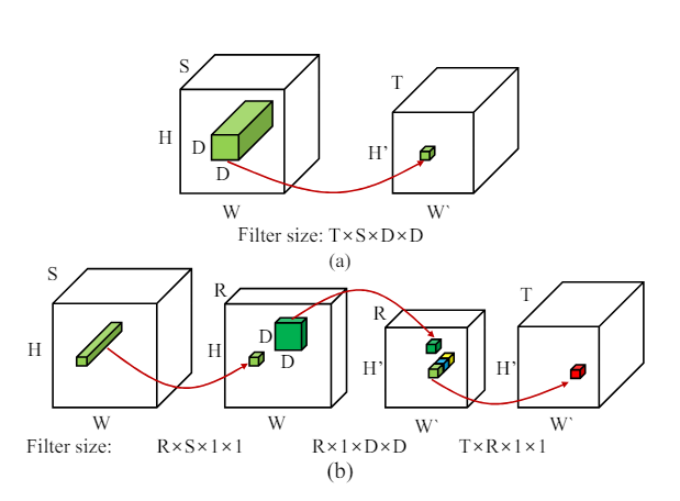
A convolution operation maps a tensor from one dimension to a tensor of another (possibly) lower dimension. If we consider an input tensor of size then a convolution layer will map this to a tensor, of size using a kernel tensor, of size .

Using similar logic as defined before, the number of multiplies required for this operation in . Thus a convolution layer is simply a multiplication operation over a subset of a tensor yielding a smaller tensor. We can approximate the kernel using a series of "smaller" multiplication operations by reducing the dimensions we need to multiply across. Consider the following decomposition,

This is similar to the case of the SVD with an important difference the core is a 4 dimensional tensor and not a matrix. Where the first term in each bracket is the size and the second term is the number of multiplies. The size is of one kernel whereas the number of multiplies is the total number of multiplies to generate the complete output (i.e. if the operation denoted by the red arrows was calculated for the entire input tensor to generate the entire output tensor, it is given by the formula, product of kernel dimensions product of output tensor dimensions ). : ( , ) : (, ) : (, ) Which makes the transformation function (with number of multiplies),

The number of multiplies in this operation is which is less than if and .

In the figure above each of the red arrows indicates a one convolution operation, in figure (a) you have one fairly large filter and one convolution, whereas in the figure (b) you have 3 convolution operations using 3 smaller filters. Let’s break down the space and size savings for this. Recall, for our fully connected layers this formula was,

Rank Selection

So we are ready to go with a decomposition, all that remains is finding out the optimal rank. Again, if the rank is too low we end up with high compression but possibly low accuracy, and if the rank is too high we end up with very low compression. In embedded systems we need to be quite aggressive in compression since this can be a hard constraint on solving a problem. In our previous example, we could "locally" optimize rank but in the case of CNNs this is not possible since at the very least we would have at least one FC and one convolutional layer and we must compress both somewhat simultaneously. Brute force quickly becomes hard, as for even modest tensor combinations such as and we can end up with far too many combinations to try. Binary search is also not possible since it is not clear if simultaneously lowering both ranks lowers accuracy.

Naive Rank Selection Algorithm

The intuition is that if a layer is more sensitive to decomposition it should have higher ranks. Our algorithm is proprietary but the intuition is as follows. We start with a rank of 1 and increase the rank by 1 until the accuracy drops below a certain threshold. We then decrease the rank by 1 and continue until the accuracy drops below a certain threshold. We then take the rank that gave the highest accuracy. This is a naive algorithm and can be improved upon.

Motivation

As someone who implements deep learning models on embedded systems, an important consideration is often the size of the model.
There are several notions of size, but the two major ones are :

• Number of elements to save, usually in the form of a matrix or tensor.
• Number of operations to perform, usually in the form of a matrix multiplication.
  The first affects the amount of memory required to store the model, while the second affects the amount of computation required to run the model.

I have worked extensively in matrix factorization before, mostly factorizing sparse matrices for recommendation systems.
Unfortunately, while there are many LoRA walk throughs using code, I was not able to find a simple succint explanation of the problem and the solution. And why it works. This article aims to address that gap by providing an elementary explanation of the problem, how to set up the optimization problem and how to solve it, in possibly linear time.
This is part I, that deals with factorizing a fully connected layer. Part II will deal with factorizing a convolutional layer.

Code Follow Along

The Jupyter Notebook for this is at https://github.com/FranciscoRMendes/tensor-rank

Introduction to Matrices

First we start with basic definitions of matrices and tensors.
If you are reading this article you probably know what a matrix is, but here is one anyway.

Again, consider a matrix multiplication with a vector,

see addendum for a tensor multiplication.

Size

Given the matrix above the main focus of this article will be to reduce the matrix size so that we never actually store all 12 elements of the matrix. With that said here is a more precise definition of how much space the matrix above takes on hardware memory.
In IEEE 754 single-precision format:

• 1 bit is used for the sign (positive or negative).
• 8 bits are used for the exponent.
• 23 bits are used for the significand (also called mantissa or fraction).

The total of 32 bits (or 4 bytes) is used to represent a single floating-point number.
So for this above matrix we need 12 memory locations or bytes. So if you were to save this matrix on a piece of hardware it would take up 4 bytes. The same applies for a tensor with 12 elements, which looks like this,

While it is useful to think of tensors as a list of matrices, it is important to note that they have some important differences as mathematical objects. It is perhaps more useful to think of matrices as a “special case” of a tensor.
For this introduction, we will stick to matrices. In a following article, I will build the equivalent intuition but for tensors. However, I will provide points of equivalence between the two, wherever possible.

Number of Operations

For the given operation, we’re performing a matrix multiplication of a 3×43×4 matrix with a 4×14×1 column vector. The resulting matrix will be a 3×13×1 column vector.

To compute each element of the resulting vector, we perform the dot product of each row of the matrix with the column vector. Since each row has 4 elements, this involves 4 multiplications and 3 additions.

Therefore, for the entire operation:

• There are 3 rows in the matrix.
• For each row, there are 4 multiplications and 3 additions.

Hence, the total number of multiplications is 3×4=123×4=12, and the total number of additions is 3×3=93×3=9.

So, in total, there are 12 multiplications and 9 additions involved in the matrix-vector multiplication operation. For two matrices being multiplied of dimensions and , there are multiplications. And the number of additions is . Notice that the number of multiplies is always greater than the number of sums.

Neural Networks as sequences of matrix/ tensor operations

A Neural Network is simply a sequence of tensor operations. In this section we will outline a simple neural network and illustrate this concept.
Input (3 nodes) –> Hidden Layer (2 nodes, ReLU) –> Output Layer (2 nodes, Sigmoid)

Hidden layer:

Output layer:

We can combine these equations into one :

In embedded systems its common to just feed an extra input of 1’s to the input and drop the biases. If you are familiar with matrix formulations of linear regression, you are probably familiar with this, but if not, you can see this clearly by the following,

Thus, after adding in the 1s to X and the column of biases to we get,

This X and W are modified versions of the X, W mentioned before but we will stick to this notation for the rest of this article. You can generalize this to as many layers as you want.

Computational Complexity and Size

Recall that we already defined how much memory is occupied by a matrix. So our matrix requires 6 x 4bytes of memory. For simplicity I will only refer to the number of elements i.e. 6.
To give you a sense of how big this can be consider an input of 8192 FFT coefficients, and a second layer of size , . On embedded systems everything is always a power of two (I wonder why). Number of multiplies is
number of additions (see above).
For a signal/ image processing problem, usually

Since our input data is usually either images or signals of the order of etc but the classes are usually several orders of magnitude smaller usually but at most . This is usually a very small matrix.

Simpler Problem Statement of Size Reduction

Let us start by trying to find a smaller matrix , that does the job of the bigger matrix. In more formal terms this means finding a matrix such that but where is smaller in some sense than .
Fortunately this is a very well defined problem in mathematics and can be solved by taking an SVD of and choosing the largest singular values, where (usually) where are the dimensions of .

The more perceptive of you will have noticed that we have two options to replace the matrix , we can use the fully multiplied out version or the components .

Size

First, let’s analyze the two in terms of size. The size of is the same as . What about the size of ?

Where are the dimensions of and is how many singular values were chosen.
How much space did we save?

Recall,

We can in fact, place an upper bound on for an SVD to save space.

Where usually this upper bound is never tight. In our example, this value is ,

Usually, we aim to reduce this number by 50% or more i.e. a rank of around 64. But in many of
our use cases we see ranks of the order etc. as being enough.

Multiplication

If the concept of size is clear, then it immediately becomes clear why the number of
multiplications also reduces.
When multiplying by , where has dimensions and has dimensions , each element of the resulting matrix is obtained by taking the dot product of a row from with a column from . Since has dimensions and has dimensions , each dot product involves multiplications. Therefore, the total number of multiplications for is .

Formulating The Indirect Optimization Problem

Okay so we know what to do, we need to find an that keeps the original activations as close to the original value as possible. Lets say the original activations were
I will explain later what the “indirect” means.

The new activations are

For a given metric, of distance and a given tolerance between the two activations, we have the following optimization problem,

Minimize subject to the distance between the activation values being low. Obviously the maximum distance will be when , is an aggressive low rank (=1) approximation of . And minimal distance will be when . However, it is very hard to define a good delta, since even if is low it is possible that that value gets amplified for the rest of the network. To combat this we can reformulate the problem in terms of the final prediction by plugging in to the original network leaving all the other layers unchanged. Thus we can optimize our final prediction directly. Using the equation for an arbitrary number of layers ,

Now we can use any classification metric, on the real data to measure our performance.

Thus, we need to find the smallest such that the difference in error is below the tolerance level. Note, 2 things

• The problem is easily interpret-able now, find the smallest s.t. the difference in accuracy is at most 0.1.
• Second, we is generally much larger than every other matrix in the problem, so while you could run more complex optimizations involving combinations of and finding the ranks, for each one that maintains a certain difference in accuracy. But in practice this is not necessary since the overall space savings for all the matrices are heavily dominated by the size of the first matrix. In other words, if the largest matrix is reduced in size by 70 percent and every other one is reduced in size by 98 percent, the overall space savings is still 70 percent.

Optimization Algorithm

One obvious way to do this would be a brute force approach, that is, to simply start at and choose smaller and smaller ranks and check if the constraint is satisfied. But for most of my use cases, this turned out to be too long. In our example it would mean trying all the way from to . Interestingly, where you choose to start at or at depends on where you expect to find a rank that is close enough to your desired accuracy.
There is an easier way to achieve this, but the proof is left as an exercise for the reader. Hint : study the properties of the optimization
algorithm at and and see if you can find where your next choice of should be.

Formulating the Direct Optimization Problem

The indirect optimization problem is a purely mathematical problem that does not “know” that the matrix comes from a neural network.
Now we know that the matrix comes from a neural network, we can use this information to our advantage.
Recall, the general formulation of a neural network,

We can use the fact that the matrix comes from a neural network to our advantage. We can use the loss function of the neural network to directly optimize the matrices .
Here, we must be careful to change the notation slightly. We will denote the matrices as to indicate that they are the matrices that come from the first layer of the neural network.
But these are not necessarily the matrices that come from the SVD of i.e. when we multiply them together we may not get .
The reason for this is that the neural network learns the best that minimize the loss function of the neural network, not the best that minimize the distance between the activations of the original and the new matrix.
This is a subtle but important distinction. This is the approach that LoRA uses.

LoRA optimization, where U,S and V are defined for a suitable choice of , is a direct optimization problem.

However, there are some important disadvantages to this approach. Let us start with the advantages,

• Easy to understand, we want low rank matrices instead of our first layer, so why not start with them and optimize them directly.
• The optimization problem is now a neural network optimization problem, which is a well studied field.
• Training is much faster than if you trained on a full rank matrix in the first layer. This is important if you want to run many trials with other hyperparameters.
• Binary search as known issues.
  Disadvantages,
• You need to know the rank of the matrix you are looking for. This is not always easy to know.
• If you want to find the rank you need to run the optimization problem for every rank you want to try.And this optimization problem is more expensive than the one above.
• The optimization problem is non-convex, so you may not find the global minimum for the delta you want. Randomness between runs could result in a different weight matrix every time.

Conclusion

For us a neat work around was to get a sense of a usable rank by running the indirect optimization problem and then using that rank to run the direct optimization problem. This way we could get a good rank in a reasonable amount of time.
Let us recap some of the important concepts we have learned in this article.

• The size of a matrix is the number of elements it has.
• The number of operations in a matrix multiplication is the number of multiplications and additions involved.
• The rank of a matrix is the number of linearly independent rows or columns it has.
• The SVD of a matrix is a way to factorize it into three matrices.
• The low rank approximation of a matrix is a way to approximate it with a smaller matrix.
• The low rank approximation of a matrix can be found by taking the SVD of the matrix and choosing the largest singular values.
• There are two ways to find the low rank approximation of a matrix: the indirect optimization problem and the direct optimization problem.

References

1. LoRA: Low-Rank Adaptation of Large Language Models
2. Low Rank Approximation of a Matrix
3. Singular Value Decomposition
4. Matrix Multiplication

Addendum

Tensor multiplication is a generalization of matrix multiplication. In tensor multiplication, the order of the tensors matters. For example, the product of a 3×4×2 tensor with a 2×4×1 tensor is a 3×4×1 tensor. The number of multiplications and additions involved in tensor multiplication is the same as in matrix multiplication, but the dimensions of the tensors are different. For example, the product of a 3×4×2 tensor with a 2×4×1 tensor involves 3×4×2=243×4×2=24 multiplications and 3×3=93×3=9 additions.
Example of tensor multiplication of two tensors and , for ease of exposition is actually an identity matrix.

Tensor :